Introduction
The hydromad package is designed for hydrological modelling and associated data analysis. It is focussed on a top-down, spatially lumped, empirical approach to environmental hydrology. In practice the emphasis is on models of rainfall runoff in catchments (watersheds). Such models predict streamflow from time series of areal rainfall and temperature or potential evapo-transpiration. They can be calibrated to time series of observed data.
As spatially lumped models, they do not explicitly represent spatial variation over the catchment area. In particular, the standard formulations do not attempt to model effects of changes in land cover. These models are usually calibrated to a period of observed streamflow, and the parameters defining the modelled relationship between rainfall, evaporation and flow are assumed to be stationary in this period.
The modelling framework in the hydromad package is based on a two-component structure: (1) a soil moisture accounting (SMA) module; and (2) a routing or unit hydrograph module (Figure @ref(fig:model-framework)). The SMA model converts rainfall and temperature into effective rainfall — the amount of rainfall which eventually reaches the catchment outlet as streamflow (i.e. that which is not lost as evaporation etc). The routing module converts effective rainfall into streamflow, which amounts to defining the peak response and shape of the recession curve. It is usually a linear transfer function, which can be as simple as a single exponential recession (i.e. constant decay rate), although variants with non-linearities are also available.

The modelling framework in the hydromad package.
The hydromad package is intended for:
- defining and fitting spatially-lumped hydrological models to observed data;
- simulating these models, including model state variables and component flow separation.
- evaluating and comparing these models: summarising performance by different measures and over time, using graphical displays (hydrograph, flow duration curve, residuals, etc) and statistics;
- integration with other types of data analysis and model analysis in
R, including sensitivity and uncertainty analyis.
This tutorial describes how to get started with the hydromad R package. It covers the basics of reading data in from files, converting it into the appropriate format, and fitting and analysing a simple model.
Once you have R running (See http://www.r-project.org/) and have installed the hydromad package (See http://hydromad.catchment.org/), you can load it:
Input data
The example we will look at is the Cotter River catchment at Gingera (gauge 410730) in the Australian Capital Territory, Australia. This is a 148 km\(^2\) catchment managed for urban water supply. Areal rainfall was estimated from several rain gauges operated by the Bureau of Meteorology and EcoWise. The temperature records come from Canberra Airport.
The Cotter data is built in to the hydromad package, and can be loaded into the workspace with:
data(Cotter)See Appendix @ref(reading-in-data) for a demonstration of reading in the time series data from files.
Data checking
In a real data analysis problem, data checking is a central issue. However, as this document aims to introduce the core modelling functions, only a simple check will be demonstrated here. The most obvious thing to do is to plot the time series, as shown in Figure @ref(fig:dataplot).
To plot the raw (daily) time series:
xyplot(Cotter)To plot a section of the time series:
And to plot the timeseries aggregated to a monthly timestep:
monthlyPQE <- aggregate(Cotter, as.yearmon, mean)
xyplot(monthlyPQE,
       screens = c("Streamflow (mm/day)", "Areal rain (mm/day)", "Temperature (deg. C)"),
       xlab = NULL)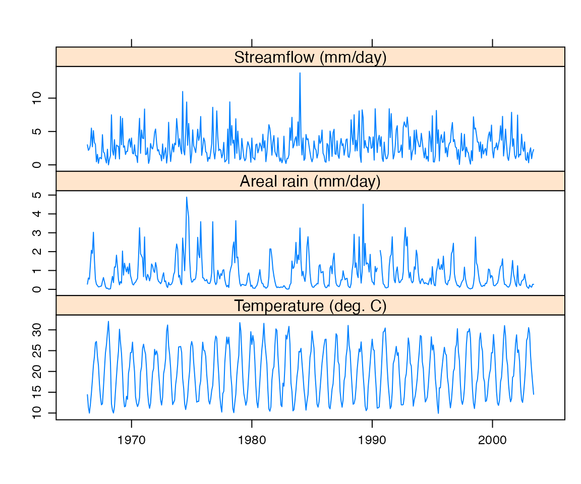
Input data, averaged over months
Table @ref(tab:datasummary) shows the mean and quartiles of each input data series. One measure that is of key interest in hydrology is the runoff ratio, the proportion of the rainfall which flows out of the catchment. In a simple case this is just sum(Q) / sum(P), but as we have missing values, we should only compare the common observations:
ok <- complete.cases(Cotter[,1:2])
with(Cotter, sum(Q[ok]) / sum(P[ok]))
## [1] 0.279101This figure is within the range we would expect, so is looks like we probably have the right data series and units.
To estimate the delay time between rainfall and a consequent streamflow response, we can look at the cross-correlation function. The hydromad function estimateDelay picks out the lag time corresponding to the maximum correlation between rainfall and rises in streamflow. In the Cotter this is 0 days. For more detail there is a function rollccf which calculates the cross-correlation in a moving window through the data, shown in Figure @ref(fig:rollccf-plot). When the cross-correlation value drops down towards zero, there is little connection between rainfall and streamflow, and you should start to worry about the data. If the lag 1 value jumps above the lag 0 value, this indicates that the delay time has changed.
x <- rollccf(Cotter)
xyplot(x, xlim = extendrange(as.Date(c("1980-01-01","1990-01-01"))))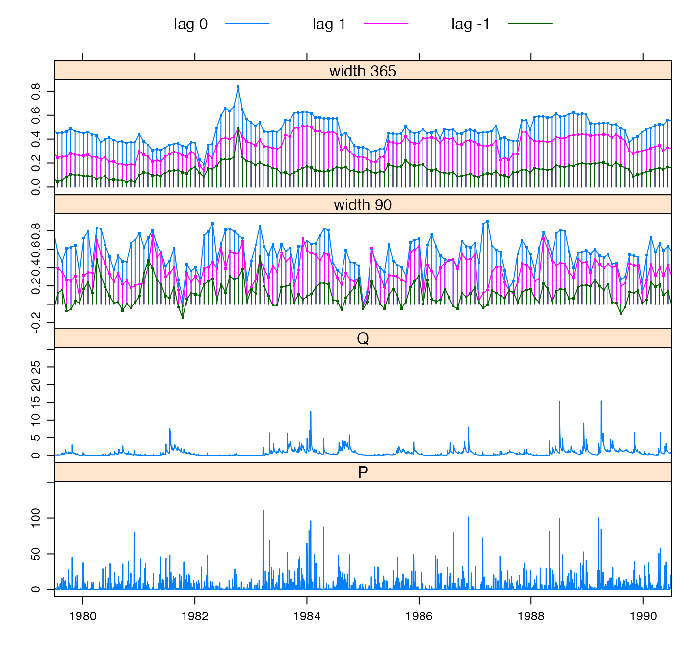
Cross-correlation between rainfall and streamflow rises, in two rolling windows of width 90 days and 365 days.
Model Specification
A hydromad object encapsulates the chosen model form, parameter values (or ranges of values), as well as results. The model form is divided into two components: SMA (Soil Moisture Accounting) and routing. Additionally, a specification can be given for fitting the routing component (rfit). If given, this is applied automatically to fit the routing component after the SMA parameters have been specified.
Let us define some data periods. We will fit a model to one, the calibration period, and then simulate it on the other periods to cross-check model performance.
ts70s <- window(Cotter, start = "1970-01-01", end = "1979-12-31")
ts80s <- window(Cotter, start = "1980-01-01", end = "1989-12-31")
ts90s <- window(Cotter, start = "1990-01-01", end = "1999-12-31")
When we first set up the model, most of the parameters are not uniquely specified, but rather have a range of possible values. These defaults are taken from hydromad.options(), and they can be over-ridden by arguments to the hydromad function.
A nice simple starting point is the classic IHACRES model of Jakeman and Hornberger (1993), which is a Soil Moisture Accounting model referred to here as "cwi" (Catchment Wetness Index).
The routing component typically used in IHACRES is a Unit Hydrograph composed of exponential components, a structure referred to here as "expuh". Up to three time constants can be specified, referred to as tau_s (slow component \(\tau_s\)), tau_q (quick component \(\tau_q\)) and tau_3. The partitioning of flow between the stores is set by v_s (fractional volume in the slow component \(v_s\)), and by default the quick flow component is assigned the remainder.1
When a model structure is specified, default parameter ranges for the given SMA model are applied, and others can be specified:
cotterMod <- hydromad(ts90s, sma = "cwi", routing = "expuh",
                      tau_s = c(5,100), tau_q = c(0,5), v_s = c(0,1))
print(cotterMod)
##
## Hydromad model with "cwi" SMA and "expuh" routing:
## Start = 1990-01-01, End = 1999-12-31
##
## SMA Parameters:
## lower upper
## tw 0 100
## f 0 8
## scale NA NA
## l 0 0 (==)
## p 1 1 (==)
## t_ref 20 20 (==)
## Routing Parameters:
## lower upper
## tau_s 5 100
## tau_q 0 5
## v_s 0 1With this model specification, we can choose to calibrate the model in various ways, or to simulate from the specified parameter space, or to run sensitivity or uncertainty analysis.
Calibration
Currently implemented calibration methods include simple sampling schemes (fitBySampling), general optimisation methods with multistart or presampling (fitByOptim) and the more sophisticated Shuffled Complex Evolution (fitBySCE) and Differential Evolution (fitByDE) methods. All attempt to maximise a given objective function.
The objective function can be specified as the objective argument to these functions, or by setting hydromad.options(objective = ). It is given as an R function which may refer to the values Q and X, representing observed and modelled flow, respectively. For more advanced use it may also refer to U (modelled effective rainfall), or the full input DATA matrix.
The nseStat function implements a generalisation of the familiar \(R^2\) coefficient of efficiency (Nash and Sutcliffe, 1970):
\[
\mathrm{nseStat}(Q,X) = \frac{ \sum |Q_* - X_*|^2 }{ \sum |Q_* - Z_*|^2 }
\] where \(Q\) and \(X\) are the observed and modelled values; \(Z\) is the result from a reference model, which is the baseline for comparison. \(Z\) defaults to the mean of observed data \(\mathrm{E}(Q_*)\), corresponding to the typical \(R^2\) statistic. Subscript \(*\) denotes transformed data, and the transform can be specified. See ?nseStat and ?hydromad.stats for examples.
Here we use the default, which is a weighted sum of the \(R^2\) of square-root transformed data, and (with less weight) the \(R^2\) of monthly-aggregated data.
For this simple example, the model will be calibrated using the fitByOptim function, which performs parameter sampling over the pre-specified ranges, selecting the best of these, and then runs an optimisation algorithm from that starting point.
cotterMod <- update(cotterMod, routing = "armax", rfit = list("sriv", order = c(n=2, m=1)))
cotterFit <- fitByOptim(cotterMod, samples = 100, method = "PORT")
See the help pages help("hydromad") and help("fitByOptim") for details of some of the options available.
Model Output
Now that we have an object representing a calibrated model, what can we do with it? There are many standard R functions which have methods for `hydromad} objects, which allow one to:
-
view model info using
print(),summary(), andobjFunVal() -
extract parameter values using
coef(). -
access data with
fitted(),residuals(), andobserved(). (These exclude the warm-up period by default.) -
run with new data using
update()orpredict(). -
simulate from parameter ranges using
simulate(). -
generate plots using
xyplot(),qqmath(), etc.
For details, see the examples below, the user manual, and the help page of each function.\footnote{Note that to get help for generic functions it is necessary to specify the method for hydromad objects: e.g. ?predict.hydromad or ?xyplot.hydromad. The help pages are also available from the web site http://hydromad.catchment.org/.
Most basically, one can extract the modelled streamflow time series with the function fitted(), and this can of course be used with any of R’s library of analysis functions. A quick way to view the modelled and observed streamflow time series together is to call xyplot() on the model object, as in Figure @ref(fig:obs-mod-plot). Examples below also show the output from calling the functions print() and summary() on the model object.
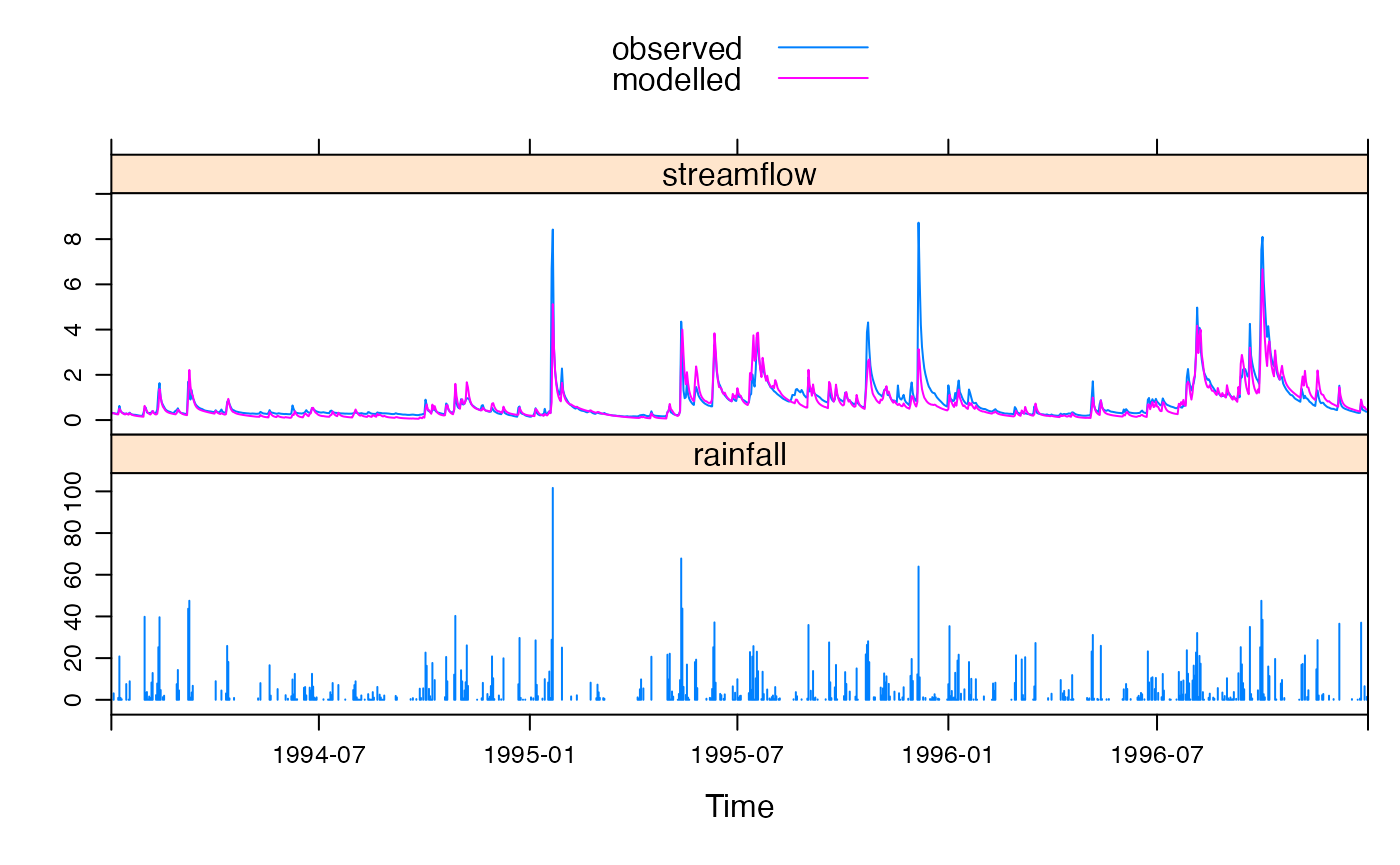
Observed vs modelled streamflow in part of the calibration period.
To display information and parameters of a model:
print(cotterFit)##
## Hydromad model with "cwi" SMA and "armax" routing:
## Start = 1990-01-01, End = 1999-12-31
##
## SMA Parameters:
## tw f scale l p t_ref
## 29.376527 1.910419 0.001693 0.000000 1.000000 20.000000
## Routing Parameters:
## a_1 a_2 b_0 b_1 delay
## 1.5236 -0.5388 0.1567 -0.1415 0.0000
## TF Structure: S + Q (two stores in parallel)
## Poles:0.558, 0.9656
##
## Fit: ($fit.result)
## fitByOptim(MODEL = cotterMod, method = "PORT", samples = 100)
## 195 function evaluations in 27.15 seconds
##
## Routing fit info: list(TRUE, 6)Note one can get hold of the parameter values using coef(cotterFit) or coef(cotterFit, which = "routing") (for the unit hydrograph only).
To display basic performance statistics for a model:
summary(cotterFit)##
## Call:
## hydromad(DATA = ts90s, tau_s = c(5, 100), tau_q = c(0, 5), v_s = c(0,
## 1), sma = "cwi", routing = "armax", rfit = list("sriv", order = c(n = 2,
## m = 1)), tw = 29.3765, f = 1.91042, scale = 0.00169348)
##
## Time steps: 3552 (33 missing).
## Runoff ratio (Q/P): (0.8179 / 3.208) = 0.2549
## rel bias: -0.03333
## r squared: 0.7733
## r sq sqrt: 0.8356
## r sq log: 0.8511
##
## For definitions see ?hydromad.statsCalculating basic performance statistics for a model. The summary function actually returns a list, containing the values of various performance statistics.
Model Simulation
We can simulate this model on the other periods using the `update function:
sim70s <- update(cotterFit, newdata = ts70s)
sim80s <- update(cotterFit, newdata = ts80s)
simAll <- update(cotterFit, newdata = Cotter)
For verification purposes, we would like to calculate performance statistics for the whole dataset but excluding the calibration period. The easiest way to do this is to set the observed streamflow data in the calibration period to `NA} (missing), and then run the simulation:
It is convenient to group these models together into a `runlist}, which is just a list of fitted models:
allMods <- runlist(calibration = cotterFit, sim70s, sim80s, simVerif)The predicted time series (hydrograph) and cumulative distribution (flow duration curve) can be generated as in Figures @ref(fig:obs-mod-plots) and @ref(fig:fdc-plot).
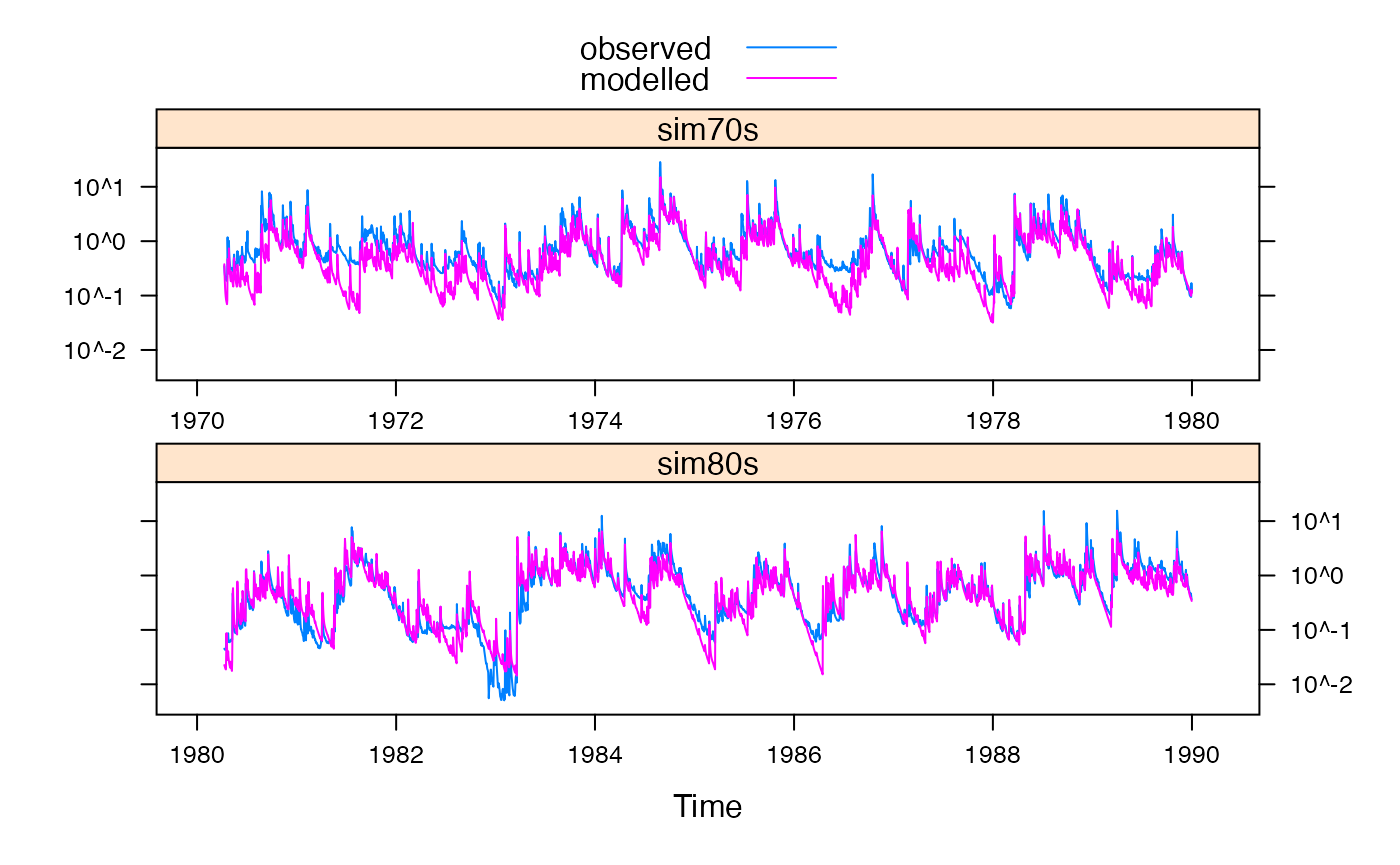
Observed vs modelled streamflow in validation periods.
summary(allMods)| rel.bias | r.squared | r.sq.sqrt | r.sq.log | |
|---|---|---|---|---|
| calibration | -0.0333273 | 0.7733200 | 0.8355996 | 0.8510658 |
| sim70s | -0.3257152 | 0.6845715 | 0.6760291 | 0.6073933 |
| sim80s | -0.1266065 | 0.7316587 | 0.8276088 | 0.8618916 |
| simVerif | -0.2082360 | 0.6936858 | 0.7530953 | 0.7547944 |
summary(simAll, breaks = "5 years")| timesteps | missing | mean.P | mean.Q | runoff | rel.bias | r.squared | r.sq.sqrt | r.sq.log | |
|---|---|---|---|---|---|---|---|---|---|
| 1966-01-01 | 1606 | 0 | 2.674010 | 0.8529382 | 0.3189735 | -0.31862832 | 0.5330459 | 0.6320879 | 0.6800752 |
| 1971-01-01 | 1826 | 0 | 3.173708 | 1.1636603 | 0.3666564 | -0.33326550 | 0.7184575 | 0.6990362 | 0.6183019 |
| 1976-01-01 | 1827 | 0 | 2.670914 | 0.7185062 | 0.2690114 | -0.22798441 | 0.6642018 | 0.7161991 | 0.6812281 |
| 1981-01-01 | 1826 | 0 | 2.914743 | 0.7902770 | 0.2711310 | -0.11380336 | 0.7752632 | 0.8424474 | 0.8612795 |
| 1986-01-01 | 1826 | 33 | 3.153246 | 0.9562480 | 0.3032583 | -0.15957919 | 0.6940339 | 0.8041123 | 0.8534372 |
| 1991-01-01 | 1826 | 0 | 3.356369 | 0.9152752 | 0.2726980 | -0.09288265 | 0.7750202 | 0.8412327 | 0.8532968 |
| 1996-01-01 | 1827 | 0 | 3.037909 | 0.6267362 | 0.2063051 | 0.14456272 | 0.7568331 | 0.8128100 | 0.8381424 |
| 2001-01-01 | 893 | 0 | 2.472430 | 0.3951501 | 0.1598226 | 0.16406907 | 0.5196486 | 0.6693259 | 0.6949333 |
| 2001-01-01 | 893 | 0 | 2.472430 | 0.3951501 | 0.1598226 | 0.16406907 | 0.5196486 | 0.6693259 | 0.6949333 |
To plot performance statistics over time:
twoYrStats <- summary(simAll, breaks = "2 years")
statSeries <- twoYrStats[,c("r.squared", "r.sq.sqrt", "rel.bias", "runoff")]
## cut off crazy R Squared values below 0 (for plotting)
statSeries[,1] <- pmax(statSeries[,1], 0)
statSeries[,2] <- pmax(statSeries[,2], 0)
c(xyplot(statSeries, type = "s", lwd = 2,
         ylab = "statistic", xlab = NULL),
  `observed streamflow` = xyplot(observed(simAll)),
  layout = c(1,5), x.same = TRUE) +
    latticeExtra::layer(panel.refline(h = 0, v = time(statSeries)), under=TRUE)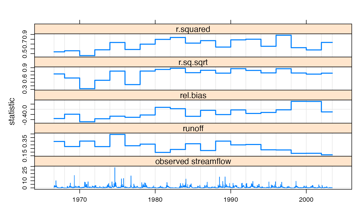
Performance statistics plotted over time in regular 2 year blocks. The runoff coefficient and observed streamflow data are also shown.
To plot the flow duration curve for modelled vs observed data in the calibration period:
To plot a flow duration curve for each of the simulated models:
qqmath(allMods, type = c("l","g"),
       scales = list(y = list(log = TRUE)),
       xlab = "Standard normal variate",
       ylab = "Flow (mm/day)",
       f.value = ppoints(100), tails.n = 50,
       as.table = TRUE)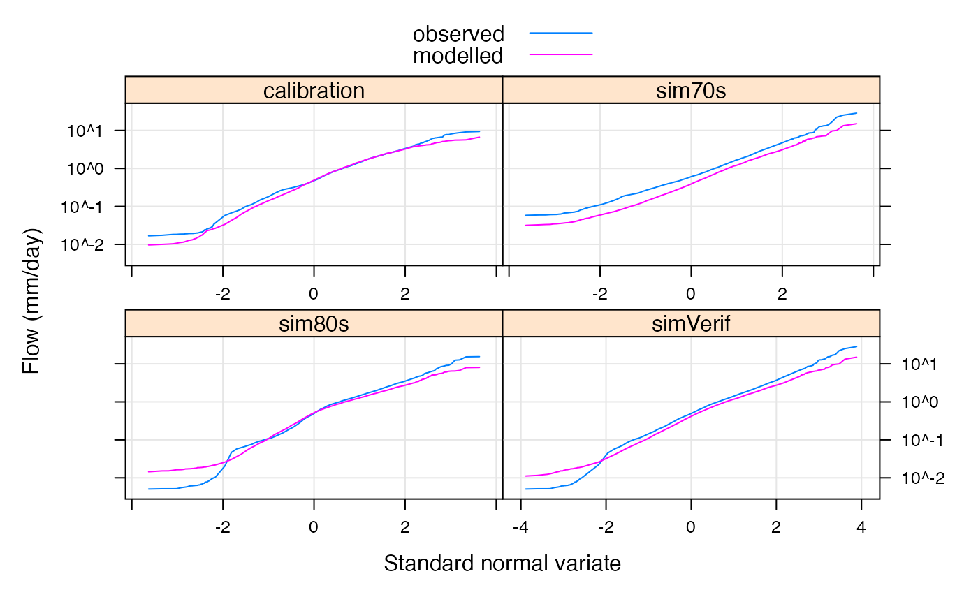
Log-normal Daily Flow Duration Curve for models in simulation.
Model and Calibration Options
There are several extensions to the basic model used so far. With different types of data, such as very dry or wet catchments, sub-daily time steps, poor areal rainfall estimates, cases of baseflow loss to groundwater, etc, different models or calibration methods will need to be used.
Model Structure and Parameter Ranges
We have used an ihacres() CWI model in this tutorial, which is a simple metric type model. Other SMA models are included in the package, or one can define a new model. See the user manual for details.
Ranges of parameters to search when calibrating the effective rainfall model can be specified as arguments to the hydromad or update() functions. Alternatively, parameters can be fixed to a given value by specifying a single number.
The default ranges can be seen, and set, using the function hydromad.options().
The example, in the CWI model, the threshold parameter l (used for intermittent or ephemeral rivers), defaults to a fixed value of 0. To allow calibration of this parameter, specify a numerical range. Similarly, the evapo-transpiration coefficient e defaults to the range \([0.01,1.5]\); to fix it to a given value, just specify it:
Optimisation settings
Each of the fitting functions has several options, and the help pages should be consulted for details. An important option is the choice of objective function; see the discussion above about how to specify it.
In the simple cases of using fitBySampling or fitByOptim, the argument samples specifies how many random parameter sets will be sampled (from the predefined parameter ranges), and argument sampletype chooses “Uniform Random”, “Latin Hypercube”, or “all combinations” (a regular grid of values). The one model with best objective function value is chosen. In the case of fitByOptim this is then improved locally with an optimisation algorithm.
Unit Hydrograph Transfer Functions
A typical unit hydrograph model, at least in models, is a linear transfer function, i.e. an ARMAX-like (Autoregressive, Moving Average, with eXogenous inputs). This can often, but not always, be formulated mathematically as a set of exponentially receding stores, which may be in a parallel and/or series configuration. ARMAX-type models are specified by the number of auto-regressive terms \(n\) and the number of moving average terms \(m\). For example, a model with one store is \((n=1,m=0)\); two stores in parallel is \((n=2, m=1)\); two stores and an instantaneous store in parallel is \((n=2, m=2)\). Three stores in parallel is \((n=3,m=2)\).
When using armax or expuh routing, specialised methods are available to estimate for calibration, such as the SRIV (Simple Refined Instrumental Variable) algorithm. These are specified using the rfit argument.
The order of the transfer function may be varied, as well as the delay time. If there is any ambiguity in choosing the best delay time, each possibility should be tried.
To test different model structures systematically, a convenience function tryModelOrders is provided. An example is given in Table @ref(tab:try-model-orders-table). In this case a simple SMA is used with fixed parameters.
For more information on these issues see, for example, Jakeman et. al. (1990) and Young (2003).
ihSpec <- hydromad(ts90s, sma = "cwi", tw = 10, f = 1,
                   routing = "armax")
osumm <- tryModelOrders(update(ihSpec, rfit = "sriv"),
                        n = 0:3, m = 0:3, delay = 0)
summary(osumm)| ARPE | r.squared | r.sq.log | |
|---|---|---|---|
| (n=0, m=0, d=0) | 0.000 | -5.432 | -2.421 |
| (n=1, m=0, d=0) | 0.000 | 0.545 | 0.705 |
| (n=1, m=1, d=0) | 0.000 | 0.671 | 0.774 |
| (n=2, m=0, d=0) | 0.015 | 0.344 | 0.550 |
| (n=2, m=1, d=0) | 0.001 | 0.694 | 0.782 |
| (n=2, m=2, d=0) | 0.005 | 0.698 | 0.782 |
| (n=3, m=0, d=0) | 0.678 | 0.605 | 0.720 |
| (n=3, m=1, d=0) | 0.023 | 0.697 | 0.782 |
| (n=3, m=2, d=0) | 28.994 | 0.698 | 0.782 |
| (n=3, m=3, d=0) | 0.001 | 0.705 | 0.785 |
Unit Hydrograph Inverse Fitting Methods
Unit Hydrograph routing models are typically fitted using least squares or SRIV algorithms, but this depends on the modelled effective rainfall, and so must be continuously re-fitted while calibrating the SMA model. One alternative is to fit the unit hydrograph to the observed streamflow data directly – though usually constrained by rainfall – and then use that as a fixed component while calibrating the SMA model. This can be done using an inverse filtering method with rfit = list("inverse", ...). (There are many options here also).
Other such inverse fitting methods are possible, e.g. average event unit hydrograph estimation, but are not currently implemented in this package.
Other Options
If model calibration is failing, you can set hydromad.options(trace = TRUE) and/or hydromad.options(catch.errors = FALSE) to track down what is happening.
It is sometimes useful to look at the model state variables, available as predict(mod, return_state = TRUE) (for the SMA model), or predict(mod, return_components = TRUE) (for the routing model), to see if they look sensible.
Some other things to try are
- using different calibration periods;
- changing the warmup period length;
- changing the optimisation method and/or settings.
What Next?
This document has described only a basic model fitting process.
Help pages are available for most functions, and these are also available online at http://hydromad.catchment.org/. There is also a set of demos: see demo(package = "hydromad") for a list.
Please discuss any problems or suggestions with the package maintainer.
Appendix
Reading in data
The required input data files for this tutorial are included with the hydromad package, in the doc directory. Note that the processed data is available directly in R – just type data(Cotter) – but this section shows how to read it in from text files as an exercise.
A few simple steps are required to import and convert the data into a usable form:
- extracting dates from the files,
- converting streamflow from ML/day to mm/day,
- handling missing data values,
- and aligning the three time series in a common time period.
Let’s first view the content of one of the input files. Set the working directory to where the data file is:
file.show("data/pq_cotter.csv")## -99,49.8405,3/01/1964
## -99,48.5998,4/01/1964
## -99,46.3199,5/01/1964
## -99,44.5028,6/01/1964
## -99,41.9241,7/01/1964
## ...There is no header in the file, but we know that the columns represent rainfall (P), streamflow (Q) and date of observation. The temperature file is similar. Knowing the format and columns we can use read.table to import the data:
## rain and flow data
pqdat <- read.table("data/pq_cotter.csv", sep = ",",
                    col.names = c("P", "Q", "Date"), as.is = TRUE)
## temperature data
tdat <- read.table("data/t_cotter.csv", sep = ",",
                   col.names = c("T", "Date"), as.is = TRUE)
and view the structure of the resulting data frames:
str(pqdat)## 'data.frame': 15339 obs. of 3 variables:
## $ P : num -99 -99 -99 -99 -99 -99 -99 -99 -99 -99 ...
## $ Q : num 49.8 48.6 46.3 44.5 41.9 ...
## $ Date: chr "3/01/1964" "4/01/1964" "5/01/1964" "6/01/1964" ...
str(tdat)## 'data.frame': 15467 obs. of 2 variables:
## $ T : num 28.8 29.4 32.8 35.7 37.2 22.9 25.5 23.8 23.7 24.9 ...
## $ Date: chr "3/01/1964" "4/01/1964" "5/01/1964" "6/01/1964" ...So far, the Date columns are only text; R does not know they are dates. We need to specify the date format, where \%d is day, \%m is month number, \%b is month name, \%Y is four-digit year and \%y is two-digit year (see ?strptime).
If the day, month and year were in separate columns of the file, with names "day", "mon" and "yr" then you could do something like:
If you have sub-daily time steps, a good choice is to use the chron() function from the chron package to represent the time index.2
Negative values (-99) in the pq input file represent missing data; in R they should be set to the special value NA. Also, some dates in the temperature file are blank, and need to be removed.
The hydromad model fitting functions require that rainfall and streamflow are given in the same units, typically mm / day. The streamflow data in our input file is measured in ML / day, so we need to convert it, supplying the catchment area of 148 km\(^2\).
pqdat$Q <- convertFlow(pqdat$Q, from = "ML", area.km2 = 148)For simple applications, when the data series are already synchronised, this data frame (or matrix) format may be enough. However, there are benefits in working with actual time series objects: because they handle observation times, they allow powerful merging, treatment of missing values, rolling averages and other functions. While R has a built-in structure for regular time series (ts), these do not handle specific dates or times, only index numbers. It is recommended to work with zoo objects (using the zoo package).^[zoo objects are a generalisation of ts objects and in many cases can be used in the same way; see vignette("zoo").}
library(zoo)
tsPQ <- zoo(pqdat[,1:2], pqdat$Date, frequency = 1)
tsT <- zoo(tdat[,1], tdat$Date, frequency = 1)
We can now merge the time series together into a final dataset. Note that the hydromad package expects temperature or evapo-transpiration data to be called E, not T. 3
Cotter <- merge(tsPQ, E = tsT, all = FALSE)Print the first few rows (the head) of the time series, to check that everything looks OK:
head(Cotter, 6)## P Q E
## 1964-01-03 NA 0.3367601 28.8
## 1964-01-04 NA 0.3283770 29.4
## 1964-01-05 NA 0.3129723 32.8
## 1964-01-06 NA 0.3006946 35.7
## 1964-01-07 NA 0.2832709 37.2
## 1964-01-08 NA 0.2909014 22.9## [1] "1964-01-03" "2005-12-31"This shows that the rainfall data has missing values at the beginning. At the other end of the series, Streamflow data is missing. This will not cause a problem, but let us tidy it up anyway:
Cotter <- na.trim(Cotter)The final dataset extends from 1966-05-01 to 2003-06-12, and is shown in Figure @ref(fig:dataplot) and Table @ref(tab:datasummary):
summary(Cotter)| P | Q | E | |
|---|---|---|---|
| Min. | 0.000000 | 0.0050657 | 2.80000 |
| 1st Qu. | 0.000000 | 0.2273834 | 14.00000 |
| Median | 0.000000 | 0.4836848 | 19.20000 |
| Mean | 2.965781 | 0.8268533 | 19.69359 |
| 3rd Qu. | 1.650000 | 1.0391858 | 24.60000 |
| Max. | 141.390000 | 28.4952703 | 42.20000 |
| NA’s | 0.000000 | 33.0000000 | 0.00000 |
Computational details
The results in this paper were obtained using R 4.1.2 with the packages hydromad 0.9–27, zoo 1.8–9 and latticeExtra 0.6–29. R itself and all packages used are (or will be) available from CRAN at http://CRAN.R-project.org/.