Plot methods for Hydromad model objects

Plot methods...

# S3 method for hydromad
plot(x, y, ...)

# S3 method for hydromad
xyplot(
  x,
  data = NULL,
  ...,
  scales = list(),
  feasible.bounds = FALSE,
  col.bounds = "grey80",
  border = "grey60",
  alpha.bounds = 1,
  all = FALSE,
  superpose = TRUE,
  with.P = FALSE,
  type = "l",
  type.P = c("h", if ("g" %in% type) "g"),
  layout = c(1, NA)
)

# S3 method for hydromad.runlist
xyplot(
  x,
  data = NULL,
  ...,
  scales = list(),
  all = FALSE,
  superpose = FALSE,
  with.P = FALSE,
  type = "l",
  type.P = c("h", if ("g" %in% type) "g"),
  layout = c(1, NA)
)

# S3 method for hydromad
qqmath(
  x,
  data = NULL,
  ...,
  all = FALSE,
  type = "l",
  auto.key = list(lines = TRUE, points = FALSE),
  f.value = ppoints(100),
  tails.n = 100
)

# S3 method for hydromad
tsdiag(object, gof.lag, ...)

Arguments

x

an object of class hydromad.

y

Placeholder for plot.hydromad

...

further arguments passed on to xyplot.zoo or qqmath.

data

ignored.

scales

Placeholder

feasible.bounds

if TRUE, then ensemble simulation bounds are extracted and plotted. This only works if a feasible set has been specified using defineFeasibleSet or the update method. Note that the meaning depends on what value of glue.quantiles was specified to those methods: it might be the overall simulation bounds, or some GLUE-like quantile values.

col.bounds, border, alpha.bounds

graphical parameters of the ensemble simulation bounds if feasible.bounds = TRUE.

all

passed to fitted() and observed().

superpose

to overlay observed and modelled time series in one panel.

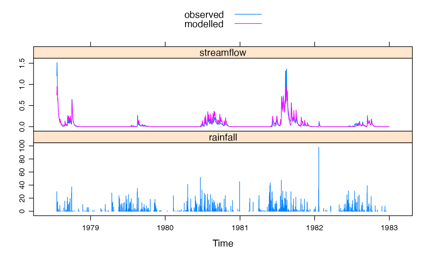
with.P

to include the input rainfall series in the plot.

type

Placeholder

type.P

plot type for rainfall, passed to panel.xyplot.

layout

Placeholder

auto.key

Placeholder

f.value, tails.n

arguments to panel.qqmath.

object, gof.lag

passed to the arima method of tsdiag.

Value

the trellis functions return a trellis object.

See also

hydromad.object, xyplot, xyplot.ts, xyplot.list

Author

Felix Andrews felix@nfrac.org

Examples

data(Canning)
cannCal <- window(Canning, start = "1978-01-01", end = "1982-12-31")
mod <-
  hydromad(cannCal,
    sma = "cwi", tw = 162, f = 2, l = 300,
    t_ref = 0, scale = 0.000284,
    routing = "expuh", tau_s = 4.3, delay = 1, warmup = 200
  )

xyplot(mod, with.P = TRUE)


c(
  streamflow = xyplot(mod),
  residuals = xyplot(residuals(mod, type = "h")),
  layout = c(1, 2), y.same = TRUE
)


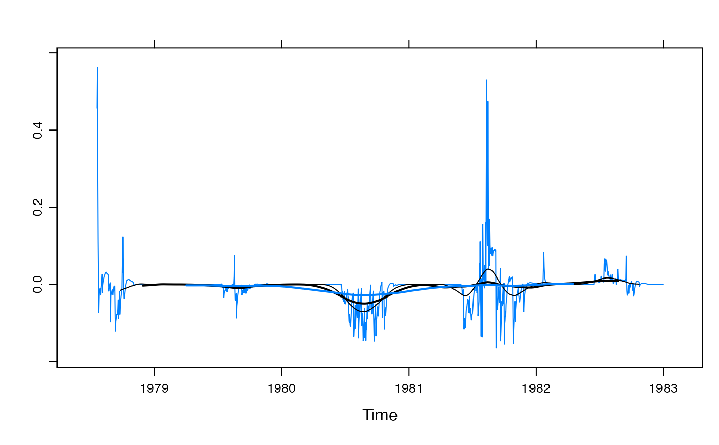
xyplot(residuals(mod)) +
  latticeExtra::layer(panel.tskernel(..., width = 90, c = 2, col = 1)) +
  latticeExtra::layer(panel.tskernel(..., width = 180, c = 2, col = 1, lwd = 2)) +
  latticeExtra::layer(panel.tskernel(..., width = 360, c = 2, lwd = 2))


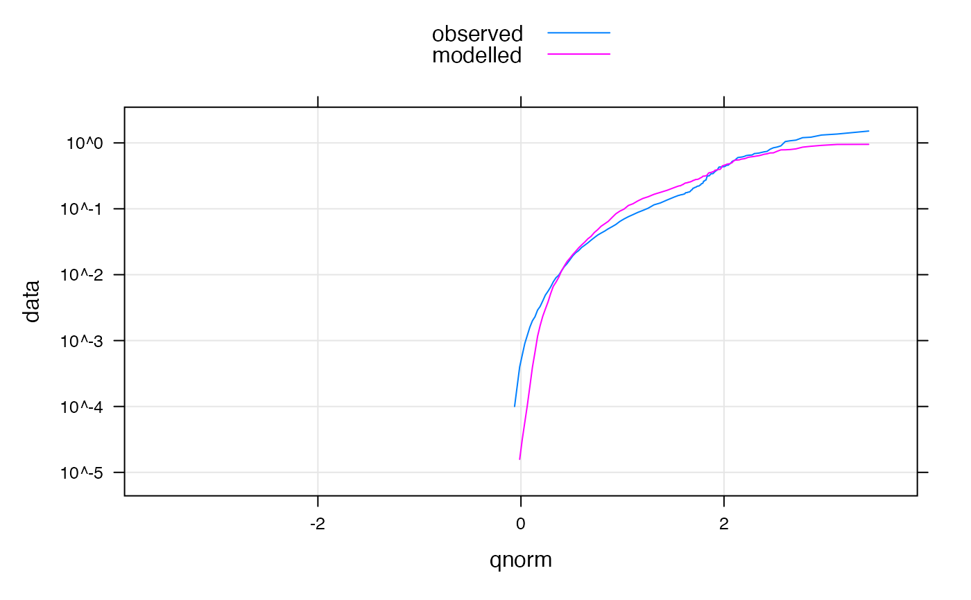
qqmath(mod,
  scales = list(y = list(log = TRUE)), distribution = qnorm,
  type = c("g", "l")
)