The HBV model included in hydromad implements the basic structure of the HBV-light by Seibert and Vis (2012). This tutorial will demonstrate how to use the hydromad HBV model and compare the output to the HBV-light model (v4.0.0.20, obtained from https://www.geo.uzh.ch/en/units/h2k/Services/HBV-Model.html).
Data requirements
Most of the required data for the model are similar to standard hydromad:
- P: timeseries of precipitation (mm)
- Q: timeseries of observed discharge (mm)
- E: timeseries of potential evapotranspiration (PET) Specifically for HBV, a further column needs to be added with:
- T: timeseries of average temperature (ºC)
If daily estimates of potential evapotranspiration are not available for your catchment, then they can be calculated using the HBV method (see equation 7 Seibert and Vis, 2012).
- A vector of length 365 with daily average PET for each day of the year
- A vector of length 12 with average daily PET for each month of the year
A vector of length 12 or 365 of mean temperature can also be provided for use in calculating PET. If it is not provided then mean monthly temperature is calculated from the timeseries of temperature. A demonstration of using the HBV PET method is provided later.
Model parameters
The structure of the model in hydromad replicates the HBV-light standard version using UZL and K0 in SUZ-box.
Snow routine
-
ttThreshold temperature for snow and snow melt in degrees Celsius. -
cfmaxDegree-day factor for snow melt (mm/(ºC.day)). -
sfcfSnowfall correction factor. Amount of precipitation below threshold temperature that should be rainfall instead of snow. -
cfrRefreezing coefficient for water in the snowpack. -
cwhLiquid water holding capacity of the snowpack.
Soil routine
-
fcMaximum amount of soil moisture storage (mm). -
lpThreshold for reduction of evaporation. Limit for potential evapotranspiration. -
betaShape coefficient in soil routine. -
cetPotential ET correction factor. Not required if PET is provided for all timesteps
In addition there is an optional flag initialise_sm to set the soil moisture store to equal fc*lp at the first timestep to match HBV-light behaviour. The default is false to match other hydromad models.
Routing routine
-
percMaximum percolation from upper to lower groundwater storage. -
uzlThreshold for quick runoff for k0 outflow (mm). -
k0Recession coefficient (quick runoff). -
k1Recession coefficient (upper groundwater storage). -
k2Recession coefficient (lower groundwater storage). -
maxbasRouting, length of triangular weighting function (days).
An additional model setting initial_slz can be used to set the initial value for the lower groundwater store (SLZ). This appears to equal the first streamflow timestep value divided by the k2 parameter in HBV-light but can be set to any value.
State variables
The following state variables can be returned from the model:
- Soil moisture accounting (
sma="hbv") module-
Snowsnow depth (mm) -
SMsoil moisture (mm) -
PETpotential evapotranspiration (mm) -
AETactual evapotranspiration (mm) -
Ueffective precipitation, or recharge, that goes to the routing module
-
- Routing (
routing="hbvrouting") module-
SUZupper groundwater storage (mm) -
SLZlower groundwater storage (mm) -
Q0quick runoff (mm) -
Q1runoff from the upper groundwater store (mm) -
Q2runoff from the lower groundwater store (mm) -
Xrouted streamflow (mm)
-
Example
This example uses the example dataset from the Corin Catchment, ACT, Australia which is included with hydromad. This dataset is a zoo object that contains daily estimates of all the required variables.
##               P      Q    E    T
## 2016-01-01 0.00 0.1152 7.87 21.4
## 2016-01-02 0.00 0.1170 4.50 17.9
## 2016-01-03 3.90 0.1264 3.97 16.1
## 2016-01-04 6.33 0.1799 2.64 13.7
## 2016-01-05 9.48 0.3879 2.41 13.7
## 2016-01-06 0.00 0.3033 3.37 14.3
Set up and fit model. If the parameters or parameter ranges are not specified then the default ranges for hbv and hbvrouting are used. These can be viewed using hbv.ranges() and hbvrouting.ranges().
mod <- hydromad(DATA = Corin,
                sma = "hbv",
                routing = "hbvrouting")
# Calibrate the default parameter ranges
fit <- fitByOptim(mod, method = "PORT")
A summary of the model fit and plot of the simulated and modelled streamflow series can be obtained as follows.
summary(fit)##
## Call:
## hydromad(DATA = Corin, sma = "hbv", routing = "hbvrouting", perc = 0.798432,
## uzl = 15.4616, k0 = 0.100156, k1 = 0.125015, k2 = 0.040413,
## maxbas = 1.50607, tt = 0.328283, cfmax = 2.27273, sfcf = 0.430303,
## cfr = 0.0191919, cwh = 0.187879, fc = 312.218, lp = 0.898577,
## beta = 2.69746)
##
## Time steps: 1361 (0 missing).
## Runoff ratio (Q/P): (0.4495 / 2.315) = 0.1942
## rel bias: -0.02689
## r squared: 0.9157
## r sq sqrt: 0.9157
## r sq log: 0.8606
##
## For definitions see ?hydromad.stats
xyplot(fit)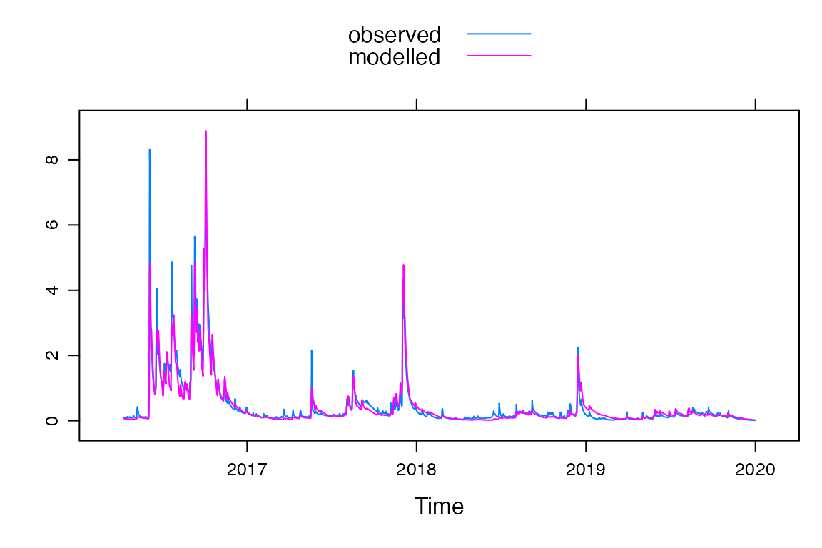
To calculate PET using the method (Seibert and Vis, 2012; equation 7), a list with named objects "PET" and "Tmean" need to be supplied to the PET argument when setting up the model. In addition, the cet parameter needs to be provided. Either a single value or a range can be provided if cet is to be calibrated.
Comparison to HBV-light
Here are some comparisons to output of the HBV-light model to ensure that correct model structures have been implemented. Comparisons are made using the Corin catchment dataset and the HBV-land dataset that comes with the HBV-light model. No warmup periods are used here to show the models produce the same results, but typically warm up periods range from 100 days (hydromad default) to a year.
Corin catchment
mod <- hydromad(DATA = Corin,
                sma = "hbv",
                routing = "hbvrouting",
                tt = 0, # Snow
                cfmax = 6.36,
                sfcf = 1,
                cfr = 0.05,
                cwh = 0.19,
                fc = 317, # Soil
                lp = 0.89,
                beta = 2.68,
                perc = 0.89, # Routing
                uzl = 71.34,
                k0 = 0.11,
                k1 = 0.15,
                k2 = 0.04,
                maxbas = 1.5,
                return_state = TRUE,
                return_components = TRUE,
                initialise_sm = TRUE,
                initial_slz = Corin$Q[1] / 0.04, # first Q timestep / k2
                warmup = 0)
The models produce the same results:
ggplot(df, aes(Date, value, col=Model)) +
  geom_line(alpha=0.5) +
  ylab("Value (mm)") +
  facet_wrap(~name, scales="free_y", ncol = 3)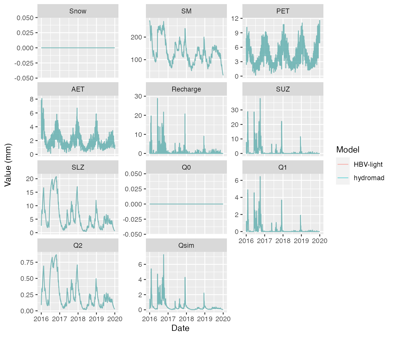
Only small rounding differences exist.
ggplot(df2, aes(Date, diff,1)) +
  geom_line() +
  ylab("Value (mm)") +
  facet_wrap(~name, ncol = 3)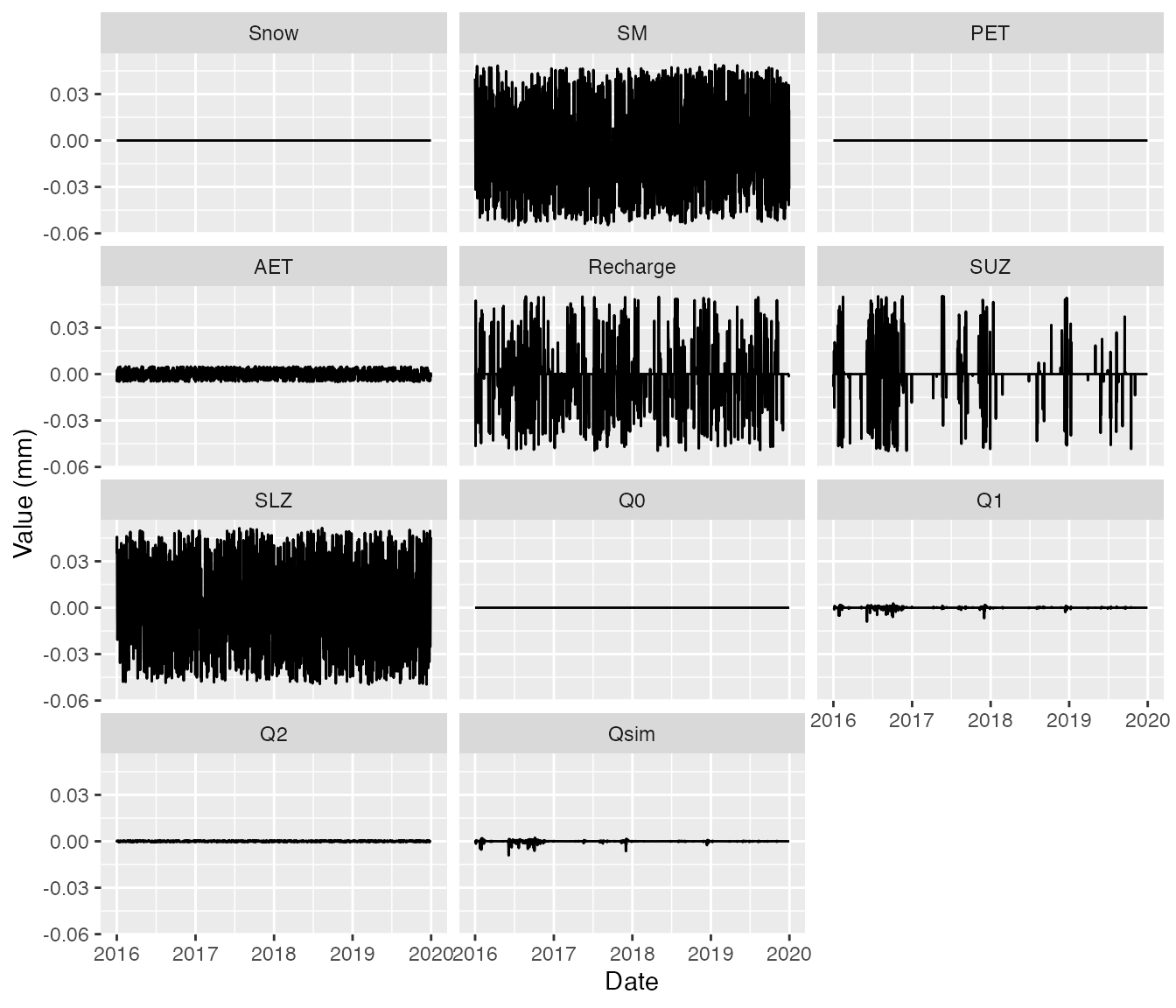
HBV-land
mod <- hydromad(DATA = hbv_land,
                sma = "hbv",
                routing = "hbvrouting",
                tt = -1.76, # Snow
                cfmax = 2.98,
                sfcf = 0.73,
                cfr = 0.05,
                cwh = 0.1,
                fc = 285, # Soil
                lp = 0.75,
                beta = 3.43,
                cet = 0.1,
                perc = 1.02, # Routing
                uzl = 17.6,
                k0 = 0.25,
                k1 = 0.09,
                k2 = 0.06,
                maxbas = 2.4,
                return_state = TRUE,
                return_components = TRUE,
                initialise_sm = TRUE,
                initial_slz = hbv_land$Q[1] / 0.06, # first Q timestep / k2
                warmup = 0,
                PET = list("PET"=hbv_land_pet, "Tmean" = hbv_land_tmean))
ggplot(df, aes(Date, value, col=Model)) +
  geom_line(alpha=0.5) +
  ylab("Value (mm)") +
  facet_wrap(~name, scales="free_y", ncol = 3)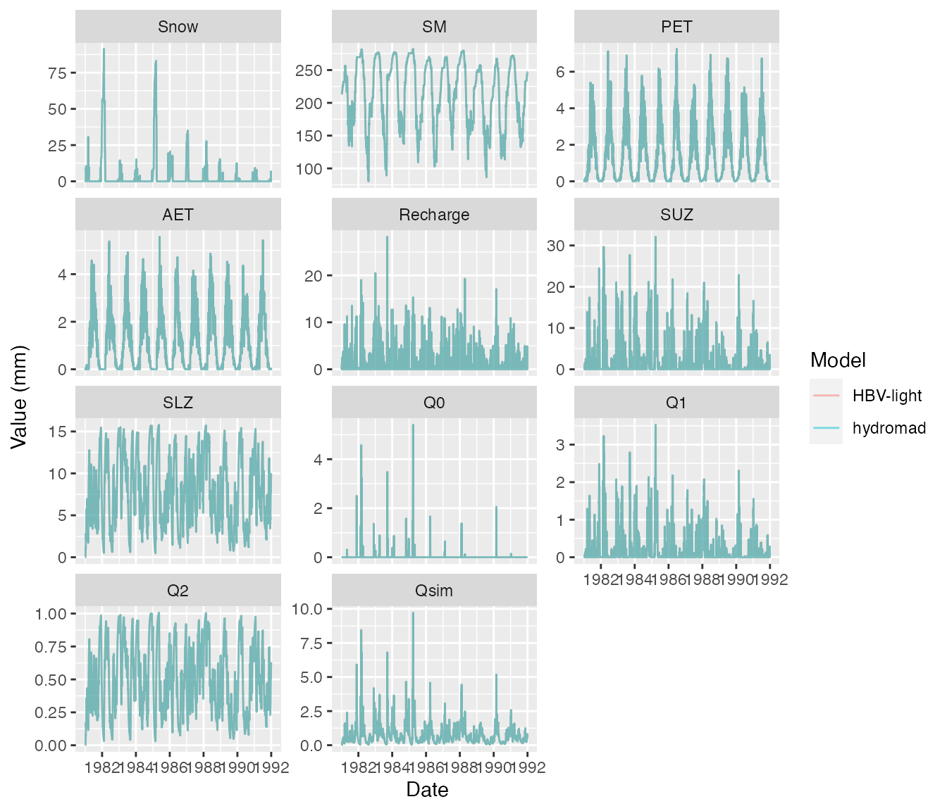
Again there are only small rounding differences.
ggplot(df2, aes(Date, diff,1)) +
  geom_line() +
  ylab("Value (mm)") +
  facet_wrap(~name, ncol = 3)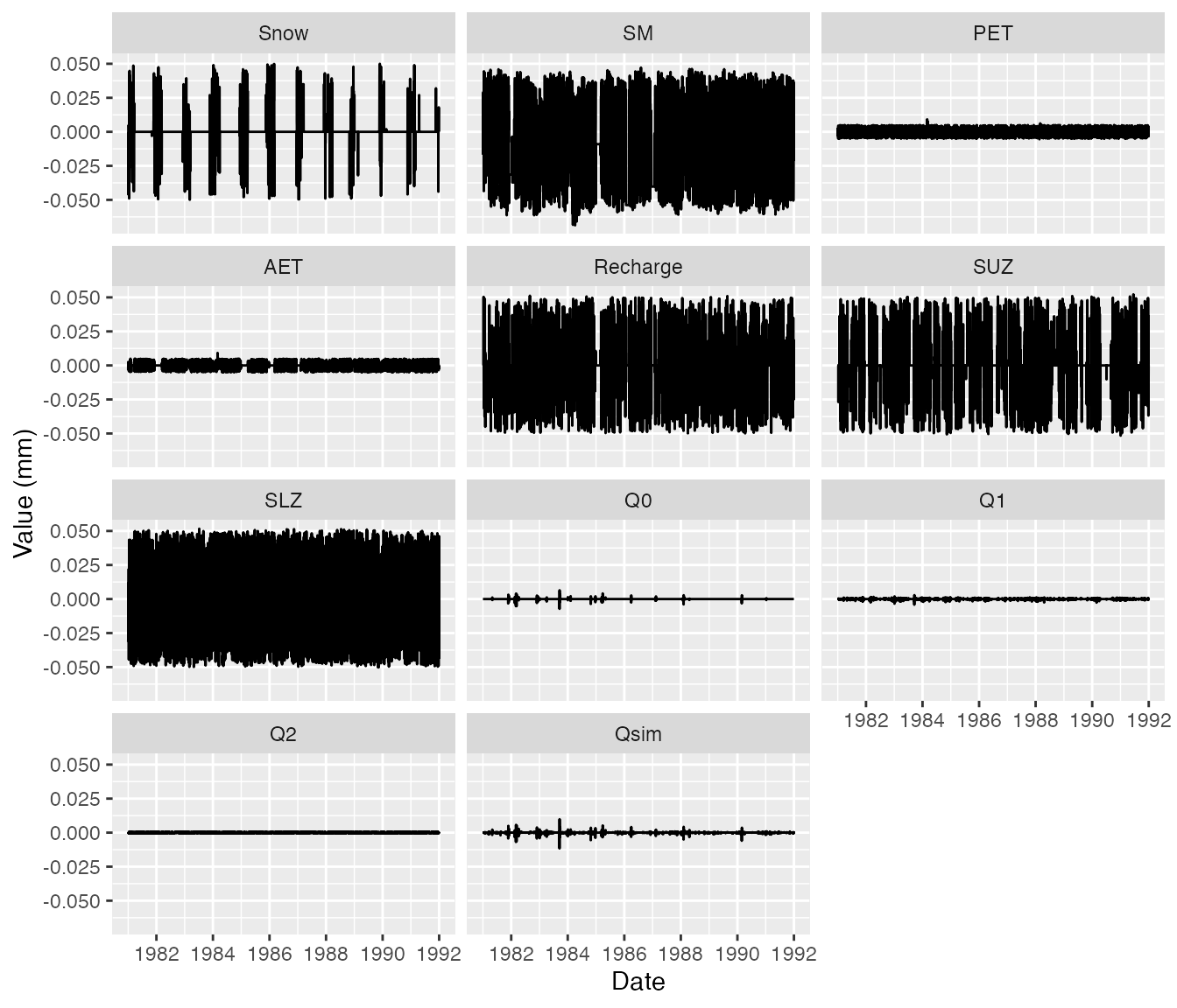
References
If you use the hydromad HBV model, you should cite the paper by Seibert and Vis, 2012 as well as the hydromad package.
- Seibert, J. and Vis, M. (2012). Teaching hydrological modeling with a user-friendly catchment-runoff-model software package. Hydrology and Earth System Sciences, 16, 3315–3325, 2012.
For additional HBV references, see:
- Bergström, S. and Forsman, A.: Development of a Conceptual Deterministic Rainfall-Runoff Model, Nordic Hydrology, 4(3), 147–170, 1973.
- Bergström, S.: The HBV Model: Its Structure and Applications,Swedish Meteorological and Hydrological Institute (SMHI), Hydrology, Norrköping, 35 pp., 1992.
- Seibert, J. (1997). Estimation of Parameter Uncertainty in the HBV Model. Hydrology Research, 28(4–5), 247–262.