The hydromad function can be used to specify models with their model
equations, data, parameters and settings. It allows a general two-component
structure, where the Soil Moisture Accounting (sma) component and the
Routing (routing) component can be arbitrary functions. A method can
be specified for fitting the dependent routing component.
hydromad(
  DATA = zoo(),
  ...,
  sma = hydromad.getOption("sma"),
  routing = hydromad.getOption("routing"),
  rfit = NULL,
  warmup = hydromad.getOption("warmup")
)
Arguments
- DATA
a
ts-like object with named columns:- list("P")
time series of areal rainfall depths, usually in mm.
- list("E")
(optional) time series of potential evapo-transpiration, or more typically, temperature as an indicator of this. Required for some models but not others.
- list("Q")
(optional) time series of discharge (streamflow) at the catchment outlet. Required for calibration but not simulation. It should usually be in units of mm (averaged over the catchment area). Use
convertFlowto convert it.- etc.
other data columns may also be included, and will be accessible via the
observed()method.
- ...
values or ranges for named parameters. Any parameters not given here will be taken from defaults given in
hydromad.options(sma)and/orhydromad.options(routing). In addition, other arbitrary arguments may be given here that will be passed on to the simulation function(s) and not treated as parameters. To specify a numeric object that is not a parameter (such as a time series object), wrap it inI().- sma
name of the Soil Moisture Accounting (SMA) component. May be
NULL, in which case the input rainfall will be passed directly torouting. Ifsmais specified, a corresponding simulation function sma.simmust exist.- routing
name of the routing component (i.e. the component which takes in effective rainfall from
smaand converts it to streamflow). May beNULL, in which case the model output is taken as the output fromsmadirectly.- rfit
optional specification for fitting the routing component. If a character string is given, then a corresponding function routing
.rfit.fitmust exist.- warmup
warmup period in number of time steps.
Value
the result from hydromad() is a
hydromad object.
Details
The hydromad() function allows models to be specified with the given
component models and parameter specifications. The resulting object can
later be modified using the update.hydromad method
using the same syntax.
Methods for working with the model objects are listed under
hydromad.object.
For a tutorial, type vignette("tutorial", package = "hydromad").
For an overview of the package, see the paper
vignette("hydromad_paper").
For a list of the package functions with their help pages, see the website http://hydromad.catchment.org/.
References
F.T. Andrews, B.F.W. Croke and A.J. Jakeman (2011). An open software environment for hydrological model assessment and development. Environmental Modelling and Software 26 (2011), pp. 1171-1185. http://dx.doi.org/10.1016/j.envsoft.2011.04.006
See also
hydromad.object
Examples
data(Cotter)
x <- Cotter[1:1000]
## IHACRES CWI model with exponential unit hydrograph
## an unfitted model, with ranges of possible parameter values
modx <- hydromad(x,
sma = "cwi", routing = "expuh",
tau_s = c(2, 100), v_s = c(0, 1)
)
modx
#>
#> Hydromad model with "cwi" SMA and "expuh" routing:
#> Start = 1966-05-01, End = 1969-01-24
#>
#> SMA Parameters:
#> lower upper
#> tw 0 100
#> f 0 8
#> scale NA NA
#> l 0 0 (==)
#> p 1 1 (==)
#> t_ref 20 20 (==)
#> Routing Parameters:
#> lower upper
#> tau_s 2 100
#> v_s 0 1
## now try to fit it
fitx <- fitByOptim(modx)
fitx
#>
#> Hydromad model with "cwi" SMA and "expuh" routing:
#> Start = 1966-05-01, End = 1969-01-24
#>
#> SMA Parameters:
#> tw f scale l p t_ref
#> 100.00000 4.82739 0.00129 0.00000 1.00000 20.00000
#> Routing Parameters:
#> tau_s v_s
#> 25.2354 0.9253
#> TF Structure: single store + instantaneous in parallel
#> Poles:0.9611
#>
#> Fit: ($fit.result)
#> fitByOptim(MODEL = modx)
#> 163 function evaluations in 8.052 seconds
summary(fitx)
#>
#> Call:
#> hydromad(DATA = x, tau_s = 25.2354, v_s = 0.925311, sma = "cwi",
#> routing = "expuh", tw = 100, f = 4.82739, scale = 0.00129012)
#>
#> Time steps: 900 (0 missing).
#> Runoff ratio (Q/P): (0.7028 / 2.285) = 0.3075
#> rel bias: -7.108e-17
#> r squared: 0.7134
#> r sq sqrt: 0.8295
#> r sq log: 0.8429
#>
#> For definitions see ?hydromad.stats
#>
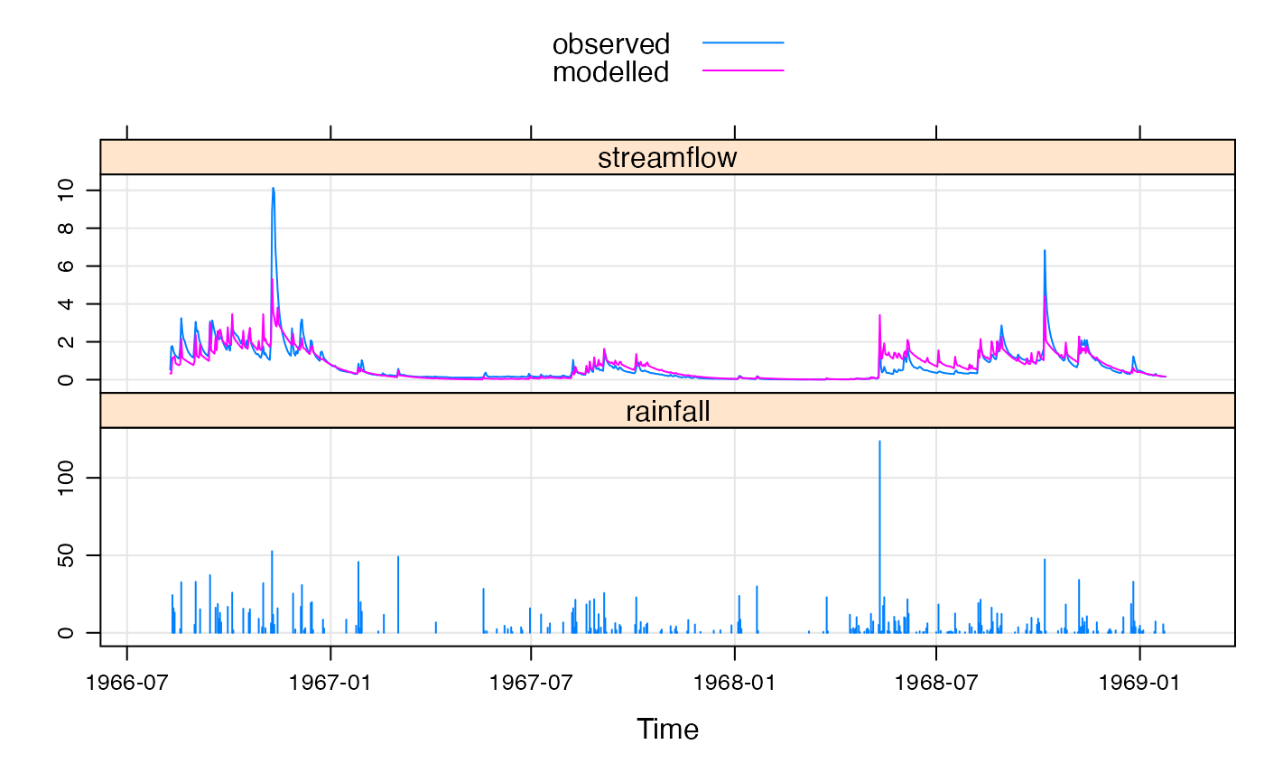
xyplot(fitx, with.P = TRUE, type = c("l", "g"))
 data(Canning)
x <- window(Canning, start = "1980-01-01", end = "1982-01-01")
xyplot(x)
data(Canning)
x <- window(Canning, start = "1980-01-01", end = "1982-01-01")
xyplot(x)
 ## IHACRES CWI model with extra parameter l
## Fixed UH (fit once) by inverse method
## an unfitted model, with ranges of possible parameter values
mod0 <- hydromad(x,
sma = "cwi", l = c(0, 100),
routing = "armax", rfit = list("inverse", order = c(1, 1))
)
#> Warning: reached maximum number of iterations
mod0
#>
#> Hydromad model with "cwi" SMA and "armax" routing:
#> Start = 1980-01-01, End = 1982-01-01
#>
#> SMA Parameters:
#> lower upper
#> tw 0 100
#> f 0 8
#> scale NA NA
#> l 0 100
#> p 1 1 (==)
#> t_ref 20 20 (==)
#> Routing Parameters:
#> a_1 b_0 b_1 delay
#> 0.8873 0.2665 -0.1538 1.0000
#> TF Structure: single store + instantaneous in parallel
#> Poles:0.8873
#>
#> Routing fit info: list(TRUE, 1)
## now try to fit the free parameters
fit1 <- fitByOptim(mod0)
fit1
#>
#> Hydromad model with "cwi" SMA and "armax" routing:
#> Start = 1980-01-01, End = 1982-01-01
#>
#> SMA Parameters:
#> tw f scale l p t_ref
#> 1.654e-02 8.000e+00 9.960e-05 1.000e+02 1.000e+00 2.000e+01
#> Routing Parameters:
#> a_1 b_0 b_1 delay
#> 0.8873 0.2665 -0.1538 1.0000
#> TF Structure: single store + instantaneous in parallel
#> Poles:0.8873
#>
#> Fit: ($fit.result)
#> fitByOptim(MODEL = mod0)
#> 289 function evaluations in 6.431 seconds
#>
#> Routing fit info: list(TRUE, 1)
summary(fit1)
#>
#> Call:
#> hydromad(DATA = x, l = 100, sma = "cwi", routing = "armax", rfit = list("inverse",
#> order = c(1, 1)), tw = 0.0165399, f = 8, scale = 9.96021e-05)
#>
#> Time steps: 632 (0 missing).
#> Runoff ratio (Q/P): (0.07337 / 3.252) = 0.02256
#> rel bias: -1.704e-06
#> r squared: 0.6568
#> r sq sqrt: 0.7325
#> r sq log: 0.6938
#>
#> For definitions see ?hydromad.stats
#>
xyplot(fit1)
## IHACRES CWI model with extra parameter l
## Fixed UH (fit once) by inverse method
## an unfitted model, with ranges of possible parameter values
mod0 <- hydromad(x,
sma = "cwi", l = c(0, 100),
routing = "armax", rfit = list("inverse", order = c(1, 1))
)
#> Warning: reached maximum number of iterations
mod0
#>
#> Hydromad model with "cwi" SMA and "armax" routing:
#> Start = 1980-01-01, End = 1982-01-01
#>
#> SMA Parameters:
#> lower upper
#> tw 0 100
#> f 0 8
#> scale NA NA
#> l 0 100
#> p 1 1 (==)
#> t_ref 20 20 (==)
#> Routing Parameters:
#> a_1 b_0 b_1 delay
#> 0.8873 0.2665 -0.1538 1.0000
#> TF Structure: single store + instantaneous in parallel
#> Poles:0.8873
#>
#> Routing fit info: list(TRUE, 1)
## now try to fit the free parameters
fit1 <- fitByOptim(mod0)
fit1
#>
#> Hydromad model with "cwi" SMA and "armax" routing:
#> Start = 1980-01-01, End = 1982-01-01
#>
#> SMA Parameters:
#> tw f scale l p t_ref
#> 1.654e-02 8.000e+00 9.960e-05 1.000e+02 1.000e+00 2.000e+01
#> Routing Parameters:
#> a_1 b_0 b_1 delay
#> 0.8873 0.2665 -0.1538 1.0000
#> TF Structure: single store + instantaneous in parallel
#> Poles:0.8873
#>
#> Fit: ($fit.result)
#> fitByOptim(MODEL = mod0)
#> 289 function evaluations in 6.431 seconds
#>
#> Routing fit info: list(TRUE, 1)
summary(fit1)
#>
#> Call:
#> hydromad(DATA = x, l = 100, sma = "cwi", routing = "armax", rfit = list("inverse",
#> order = c(1, 1)), tw = 0.0165399, f = 8, scale = 9.96021e-05)
#>
#> Time steps: 632 (0 missing).
#> Runoff ratio (Q/P): (0.07337 / 3.252) = 0.02256
#> rel bias: -1.704e-06
#> r squared: 0.6568
#> r sq sqrt: 0.7325
#> r sq log: 0.6938
#>
#> For definitions see ?hydromad.stats
#>
xyplot(fit1)
