Extract the feasible parameter sets meeting some criteria.
Source:R/defineFeasibleSet.R
defineFeasibleSet.RdExtract the feasible (or behavioural) parameter sets meeting some criteria. These could be used as a feasible set or to estimate prediction quantiles according to the GLUE (Generalised Likelihood Uncertainty Estimation) method.
defineFeasibleSet(x, ...)

# S3 method for hydromad
defineFeasibleSet(x, ..., thin = NA)

# S3 method for default
defineFeasibleSet(
  x,
  model,
  objseq = rep(1, NROW(x)),
  frac.within = 0,
  within.rel = 0.01,
  within.abs = 0.1,
  groups = NULL,
  FUN = sum,
  target.coverage = 1,
  threshold = -Inf,
  glue.quantiles = c(0, 1),
  ...
)
Arguments
- x
in the
hydromadmethod this is ahydromadmodel object which has been run through eitherfitBySamplingorfitByDreamto generate a large number of random parameter sets with associated objective function scores. In thedefaultmethod, the first argument (x) is a matrix of parameter values corresponding to the objective function valuesobjseq.- ...
extra arguments to the
hydromadmethod are passed on to thedefaultmethod. Extra arguments to thedefaultmethod will result in an error.- thin
interval between samples for results from DREAM. As it is a Markov Chain Monte Carlo method, the sequences should be thinned first to remove autocorrelation and achieve an efficient sample of the parameter distributions. The default thinning interval
NAuses the empirical autocorrelation. Seewindow.mcmc.- model
the
hydromadmodel object to be used to run simulations. Does not apply to thehydromadmethod.- objseq
objective function values corresponding to the parameter sets
x. This does not apply to thehydromadmethod, where it is assumed that the objective function values have already been calculated. Note thatobjseqcan be omitted if not using thetarget.coverageorthresholdarguments (i.e. if just defining an error criterion withfrac.within, within.rel, within.abs), so the original simulation run is not necessary.- frac.within, within.abs, within.rel
model simulations are only retained in the feasible set if some fraction
frac.withinof the simulated values are within a fractionwithin.relof the observed values OR within an absolute difference ofwithin.abs(typically mm/day).- groups, FUN
groupsis an optional grouping variable, of the same length as the observed data inmodel, used to aggregate the observed and fitted time series. The functionFUNis applied to each group. In this case, the error criteriafrac.within, within.rel, within.absare evaluated on the aggregated values, not the raw time series. Alsotarget.coverageapplies to the aggregated values. Typicallygroupswould be generated bycut.Date(for regular time periods) oreventseq(for events). Note that thefeasible.bounds(e.g. for plotting) in this case will be an aggregated time series, it will not correspond to the original time index. Useupdateorpredictto generate bounds on the original time index.- target.coverage
fraction of the observed values to be contained within the overall ranges of simulated values (minimum and maximum on each time step) from the feasible set of parameters. Note, this does not refer to the
glue.quantilesvalues, but to the overall maximum and minimum. The simulated values can be within the tolerance limit of observed values given bywithin.absto count as coverage.- threshold
value of the objective function (the objective function used to generate
objseq) used to define the feasible set: all parameter sets above this threshold value will be kept. Also thisthresholdvalue is subtracted from the objective function values to calculate weights whenglue.quantilesis given. If left as-Inf, it will be set to the minimum objective function value in the final feasible set.- glue.quantiles
if specified, these GLUE quantiles of the ensemble simulations will be calculated and stored. They can be extracted with
fittedand shown inxyplot. The quantiles are calcualted using thewtd.quantilefunction, and weighted according toobjseq-threshold. Ifglue.quantilesis left asc(0,1)then the overall minimum and maximum simulated values are taken on each time step, which is faster.
Value
a modified version of model, with added elements
feasible.set, feasible.scores, feasible.fitted,
glue.quantiles and feasible.threshold. Can be passed to
xyplot, fitted, predict, update, coef,
and print.
See also
predict.hydromad, update.hydromad,
fitBySampling, fitByDream
Examples
data(Queanbeyan)
ts74 <- window(Queanbeyan, start = "1974-01-01", end = "1976-12-01")
mod <- hydromad(ts74, routing = "expuh", rfit = list("inverse", order = c(2, 1)))
mod <- update(mod,
sma = "cwi",
tw = c(0, 100), f = c(0, 8), loss = c(-0.1, 0.1)
)
## Calculate the set of simulations within 15% error (or 1 mm/day) 90% of time.
## In this case we do not need to calculate objective function values
## beforehand. For GLUE quantiles, however, need to give 'objective'.
psets <- parameterSets(coef(mod), samples = 300)
#> Warning: parameters not fully specified, returning list
feas <- defineFeasibleSet(psets,
model = mod,
frac.within = 0.9, within.rel = 0.15, within.abs = 1
)
## How many of the 300 possible parameter sets were retained?
nrow(coef(feas, feasible.set = TRUE))
#> [1] 111
## View ranges of parameters in feasible set
feas
#>
#> Hydromad model with "cwi" SMA and "expuh" routing:
#> Start = 1974-01-01, End = 1976-12-01
#>
#> SMA Parameters:
#> lower upper
#> tw 0 100
#> f 0 8
#> scale NA NA
#> l 0 0 (==)
#> p 1 1 (==)
#> t_ref 20 20 (==)
#> Routing Parameters:
#> lower upper
#> tau_s 13.0292 13.0292 (==)
#> tau_q 0.5728 0.5728 (==)
#> v_s 0.4433 0.4433 (==)
#> v_q 0.5567 0.5567 (==)
#> delay 1.0000 1.0000 (==)
#> loss -0.1000 0.1000
#> Feasible parameter set:
#> tw f scale l p t_ref tau_s tau_q v_s v_q delay loss
#> lower 0.00 0 NA 0 1 20 13.03 0.5728 0.4433 0.5567 1 -0.09933
#> upper 97.66 8 NA 0 1 20 13.03 0.5728 0.4433 0.5567 1 0.10000
#>
#> Routing fit info: list(TRUE, 2)
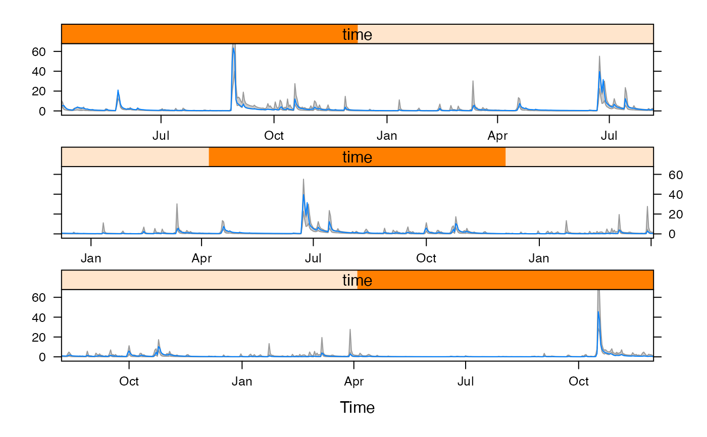
## Plot simulation bounds
xyplot(feas, feasible.bounds = TRUE, cut = 3)
 ## Generate set of simulations with NSE > 0.5, for GLUE.
## First, need to calculate objective function values:
fit <- fitBySampling(mod, samples = 300, objective = hmadstat("r.squared"))
## Calculate 5 percent and 95 percent GLUE quantiles (i.e. weighted).
fitglu <- defineFeasibleSet(fit,
threshold = 0.5,
glue.quantiles = c(0.05, 0.95)
)
## Coverage of the GLUE quantile simulations (within 0.1 mm/day)
sim <- fitted(fitglu, feasible.bounds = TRUE)
head(sim)
#> GLUE.5 GLUE.95
#> 1974-04-11 4.9134569 15.603560
#> 1974-04-12 3.9902576 12.379516
#> 1974-04-13 1.8160592 5.819653
#> 1974-04-14 1.7512514 5.715896
#> 1974-04-15 1.0651009 3.628814
#> 1974-04-16 0.7150688 2.528074
mean((sim[, 1] < observed(fitglu) + 0.1) &
(sim[, 2] > observed(fitglu) - 0.1))
#> [1] 0.8964803
## Or - keep adding parameter sets until we reach a target coverage:
## Calculate 5 percent and 95 percent GLUE quantiles (i.e. weighted).
fitglu <- defineFeasibleSet(fit,
target.coverage = 0.9,
glue.quantiles = c(0.05, 0.95)
)
## Coverage of the GLUE quantile simulations (within 0.1 mm/day)
## (not to be confused with the target.coverage to define overall feasible set)
sim <- fitted(fitglu, feasible.bounds = TRUE)
mean((sim[, 1] < observed(fitglu) + 0.1) &
(sim[, 2] > observed(fitglu) - 0.1))
#> [1] 0.800207
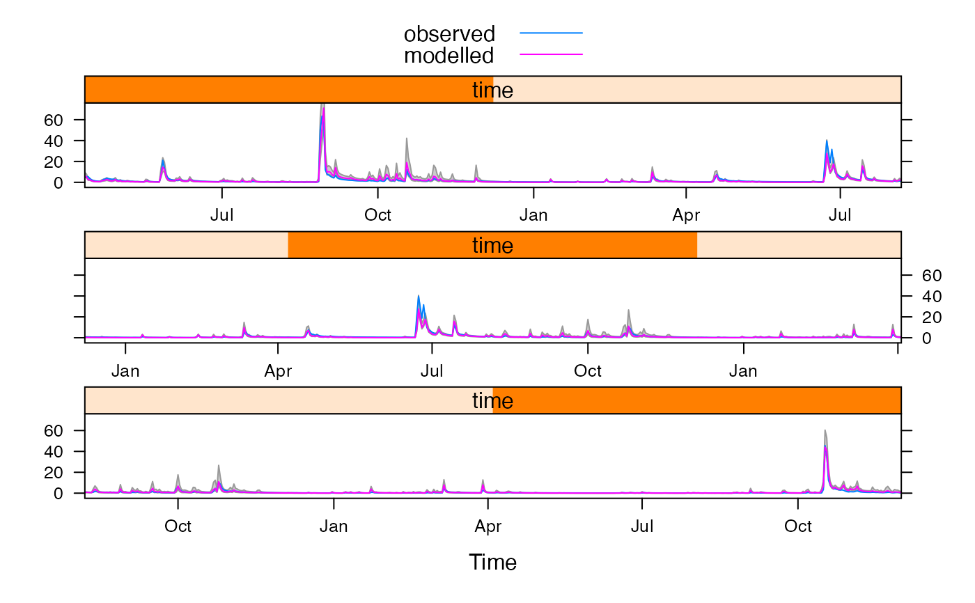
## Plot simulated GLUE quantiles
xyplot(fitglu, feasible.bounds = TRUE, cut = 3)
## Generate set of simulations with NSE > 0.5, for GLUE.
## First, need to calculate objective function values:
fit <- fitBySampling(mod, samples = 300, objective = hmadstat("r.squared"))
## Calculate 5 percent and 95 percent GLUE quantiles (i.e. weighted).
fitglu <- defineFeasibleSet(fit,
threshold = 0.5,
glue.quantiles = c(0.05, 0.95)
)
## Coverage of the GLUE quantile simulations (within 0.1 mm/day)
sim <- fitted(fitglu, feasible.bounds = TRUE)
head(sim)
#> GLUE.5 GLUE.95
#> 1974-04-11 4.9134569 15.603560
#> 1974-04-12 3.9902576 12.379516
#> 1974-04-13 1.8160592 5.819653
#> 1974-04-14 1.7512514 5.715896
#> 1974-04-15 1.0651009 3.628814
#> 1974-04-16 0.7150688 2.528074
mean((sim[, 1] < observed(fitglu) + 0.1) &
(sim[, 2] > observed(fitglu) - 0.1))
#> [1] 0.8964803
## Or - keep adding parameter sets until we reach a target coverage:
## Calculate 5 percent and 95 percent GLUE quantiles (i.e. weighted).
fitglu <- defineFeasibleSet(fit,
target.coverage = 0.9,
glue.quantiles = c(0.05, 0.95)
)
## Coverage of the GLUE quantile simulations (within 0.1 mm/day)
## (not to be confused with the target.coverage to define overall feasible set)
sim <- fitted(fitglu, feasible.bounds = TRUE)
mean((sim[, 1] < observed(fitglu) + 0.1) &
(sim[, 2] > observed(fitglu) - 0.1))
#> [1] 0.800207
## Plot simulated GLUE quantiles
xyplot(fitglu, feasible.bounds = TRUE, cut = 3)
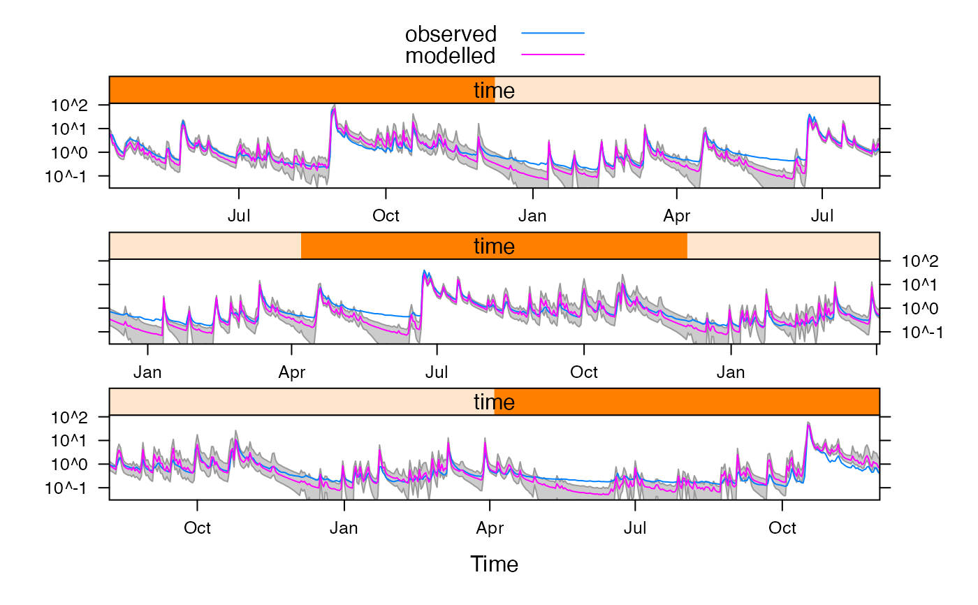
 xyplot(fitglu,
feasible.bounds = TRUE, cut = 3,
scales = list(y = list(log = TRUE))
)
xyplot(fitglu,
feasible.bounds = TRUE, cut = 3,
scales = list(y = list(log = TRUE))
)
 ## Summarise size of the simulation bounds: lower as fraction of upper
summary(coredata(sim[, 1] / sim[, 2]))
#> Min. 1st Qu. Median Mean 3rd Qu. Max.
#> 0.0000 0.1608 0.2364 0.2600 0.3643 0.8062
## Simulate on a new data period
newglu <- update(fitglu,
newdata = window(Queanbeyan,
start = "1980-01-01", end = "1982-01-01"
),
glue.quantiles = c(0.05, 0.95)
)
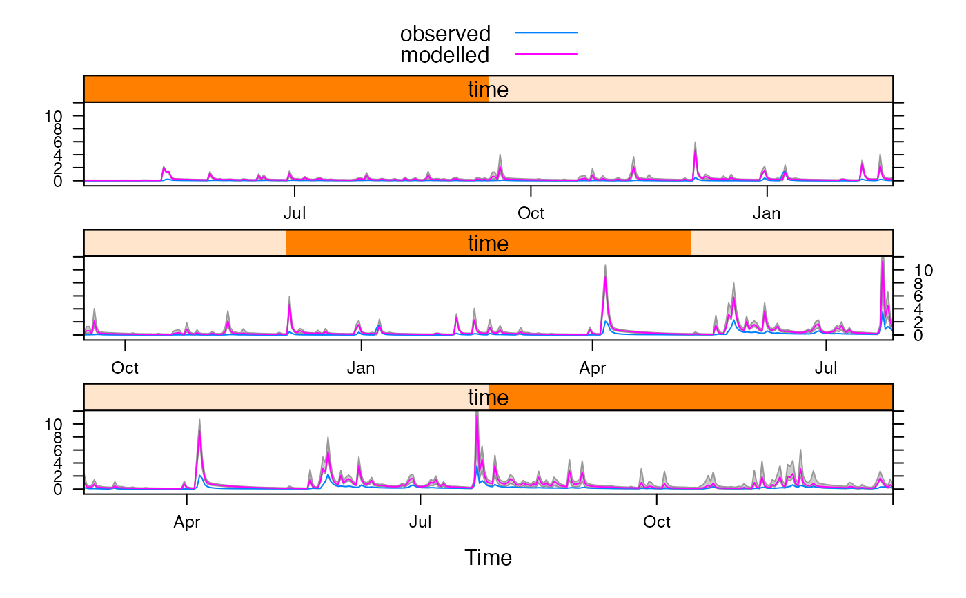
## The new period is very dry, all model simulations overestimate flow.
xyplot(newglu, feasible.bounds = TRUE, cut = 3)
## Summarise size of the simulation bounds: lower as fraction of upper
summary(coredata(sim[, 1] / sim[, 2]))
#> Min. 1st Qu. Median Mean 3rd Qu. Max.
#> 0.0000 0.1608 0.2364 0.2600 0.3643 0.8062
## Simulate on a new data period
newglu <- update(fitglu,
newdata = window(Queanbeyan,
start = "1980-01-01", end = "1982-01-01"
),
glue.quantiles = c(0.05, 0.95)
)
## The new period is very dry, all model simulations overestimate flow.
xyplot(newglu, feasible.bounds = TRUE, cut = 3)
 ## Coverage of the GLUE quantile simulations (within 0.1 mm/day)
sim <- fitted(newglu, feasible.bounds = TRUE)
mean((sim[, 1] < observed(newglu) + 0.1) &
(sim[, 2] > observed(newglu) - 0.1))
#> [1] 0.6977848
## Coverage of the GLUE quantile simulations (within 0.1 mm/day)
sim <- fitted(newglu, feasible.bounds = TRUE)
mean((sim[, 1] < observed(newglu) + 0.1) &
(sim[, 2] > observed(newglu) - 0.1))
#> [1] 0.6977848