Generalisation of Nash-Sutcliffe Efficiency (R Squared)

Generalisation of Nash-Sutcliffe Efficiency (R Squared) as a fit statistic for time series.

nseStat(
  obs,
  mod,
  ref = NULL,
  ...,
  p = 2,
  trans = NULL,
  negatives.ok = FALSE,
  na.action = na.pass
)

Arguments

obs: observed data vector.
mod: model-predicted data vector corresponding to obs.
ref: reference model predictions corresponding to obs. If NULL, ref is taken as the mean of obs after applying any transformation (trans).
...: ignored.
p: power to apply to absolute residuals (abs(obs - mod) and abs(obs - ref). The default, p = 2 corresponds to the Nash-Sutcliffe Efficiency (NSE). Setting p = 1 does not square the residuals and is sometimes called Normalised sum of Absolute Errors (NAE).
trans: a function to apply to each data series before calculating the fit statistic.
negatives.ok: if FALSE, the default case, all values in obs, mod and ref are constrained to be non-negative; i.e. negative values are replaced with zero.
na.action: a function to apply to the time series, which is expected to fill in or remove missing values (note, this is optional).

Value

a single numeric value.

Details

The result is, after transformation of variables,

$$1 - sum(abs(obs-mod)^p) / sum(abs(obs-ref)^p)$$

A perfect fit gives a value of 1 and a fit equivalent to the reference model gives a value of 0. Values less than 0 are worse than the reference model.

If the arguments obs, mod or ref are not plain vectors, nseStat will attempt to merge them together, so that corresponding time steps are compared to each other even if the time windows are not equal.

Author

Felix Andrews felix@nfrac.org

Examples


## generate some data -- it is autocorrelated so the use of these
## stats is somewhat problematic!
set.seed(0)
U <- ts(pmax(0, rgamma(200, shape = 0.1, scale = 20) - 5))
## simulate error as multiplicative uniform random
Ue <- U * runif(200, min = 0.5, max = 1.5)
## and resample 10 percent of time steps
ii <- sample(seq_along(U), 20)
Ue[ii] <- rev(U[ii])
## apply recursive filter
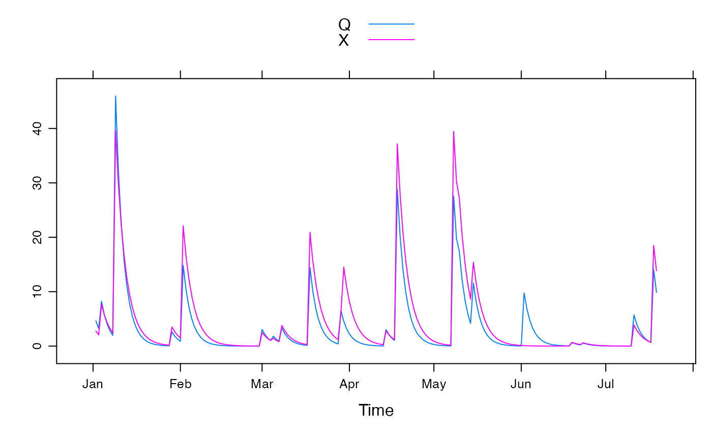
Q <- filter(U, 0.7, method = "r")
X <- filter(Ue, 0.75, method = "r")

## convert to 'zoo' objects with Date index
Q <- zoo(Q, as.Date("2000-01-01") + 1:200)
X <- zoo(X, time(Q))

xyplot(merge(Q, X), superpose = TRUE)


nseStat(Q, X)
#> [1] 0.7717829

nseStat(Q, X, trans = sqrt)
#> [1] 0.7659478

nseStat(Q, X, trans = function(x) log(x + 1))
#> [1] 0.7479644

## use absolute residuals rather than squared residuals
nseStat(Q, X, p = 1)
#> [1] 0.5564602

## use a different reference model (one-step-ahead forecast)
nseStat(Q, X, ref = lag(Q, -1))
#> [1] 0.6718251

## reference as seasonal averages rather than overall average
nseStat(Q, X, ref = ave(Q, months(time(Q))))
#> [1] 0.7534322

## see how the reference model performs in terms of R Squared
nseStat(Q, ave(Q, months(time(Q))))
#> [1] 0.0744246