Calibrate unit hydrograph transfer function models (armax or
expuh) using Least Squares with prefiltering.
armax.ls.fit(
  DATA,
  order = hydromad.getOption("order"),
  delay = hydromad.getOption("delay"),
  prefilter = hydromad.getOption("prefilter"),
  warmup = hydromad.getOption("warmup"),
  normalise = FALSE,
  fixed.ar = NULL,
  weights = NULL,
  initX = TRUE,
  na.action = na.pass,
  trace = hydromad.getOption("trace")
)
Arguments
- DATA
a
ts-like object with named columns:- list("U")
observed input time series.
- list("Q")
observed output time series.
- order
the transfer function order. See
armax.- delay
delay (lag time / dead time) in number of time steps. If missing, this will be estimated from the cross correlation function.
- prefilter
placeholder
- warmup
placeholder
- normalise
placeholder
- fixed.ar
placeholder
- weights
placeholder
- initX
placeholder
- na.action
placeholder
- trace
placeholder (i.e. negative or imaginary poles) are detected.
Value
a tf object, which is a list with components
- coefficients
the fitted parameter values.
- fitted.values
the fitted values.
- residuals
the residuals.
- delay
the (possibly fitted) delay time.
Details
In normal usage, one would not call these functions directly, but rather
specify the routing fitting method for a hydromad model using
that function's rfit argument. E.g. to specify fitting an
expuh routing model by least squares one could write
hydromad(..., routing = "expuh", rfit = "ls")
which uses the default order, hydromad.getOption("order"), or
hydromad(..., routing = "expuh", rfit = list("ls", order = c(2,1))).
References
Jakeman
See also
Examples
U <- ts(c(0, 0, 0, 1, rep(0, 30), 1, rep(0, 20)))
Y <- expuh.sim(lag(U, -1), tau_s = 10, tau_q = 2, v_s = 0.5, v_3 = 0.1)
set.seed(0)
Yh <- Y * rnorm(Y, mean = 1, sd = 0.2)
fit1 <- armax.ls.fit(ts.union(U = U, Q = Yh),
  order = c(2, 2), warmup = 0
)
fit1
#>
#> Unit Hydrograph / Linear Transfer Function
#>
#> Call:
#> armax.ls.fit(DATA = ts.union(U = U, Q = Yh), order = c(2, 2),
#>     warmup = 0)
#>
#> Order: (n=2, m=2)  Delay: 1
#> ARMAX Parameters:
#>       a_1        a_2        b_0        b_1        b_2
#>  1.249502  -0.324895   0.349207  -0.266033  -0.002811
#> Exponential component parameters:
#>     tau_s      tau_q        v_s        v_q        v_3
#>  7.859172   1.002996   0.625975   0.448592  -0.008654
#> TF Structure: S + Q + inst. (three in parallel)
#>     Poles:0.369, 0.8805
#>
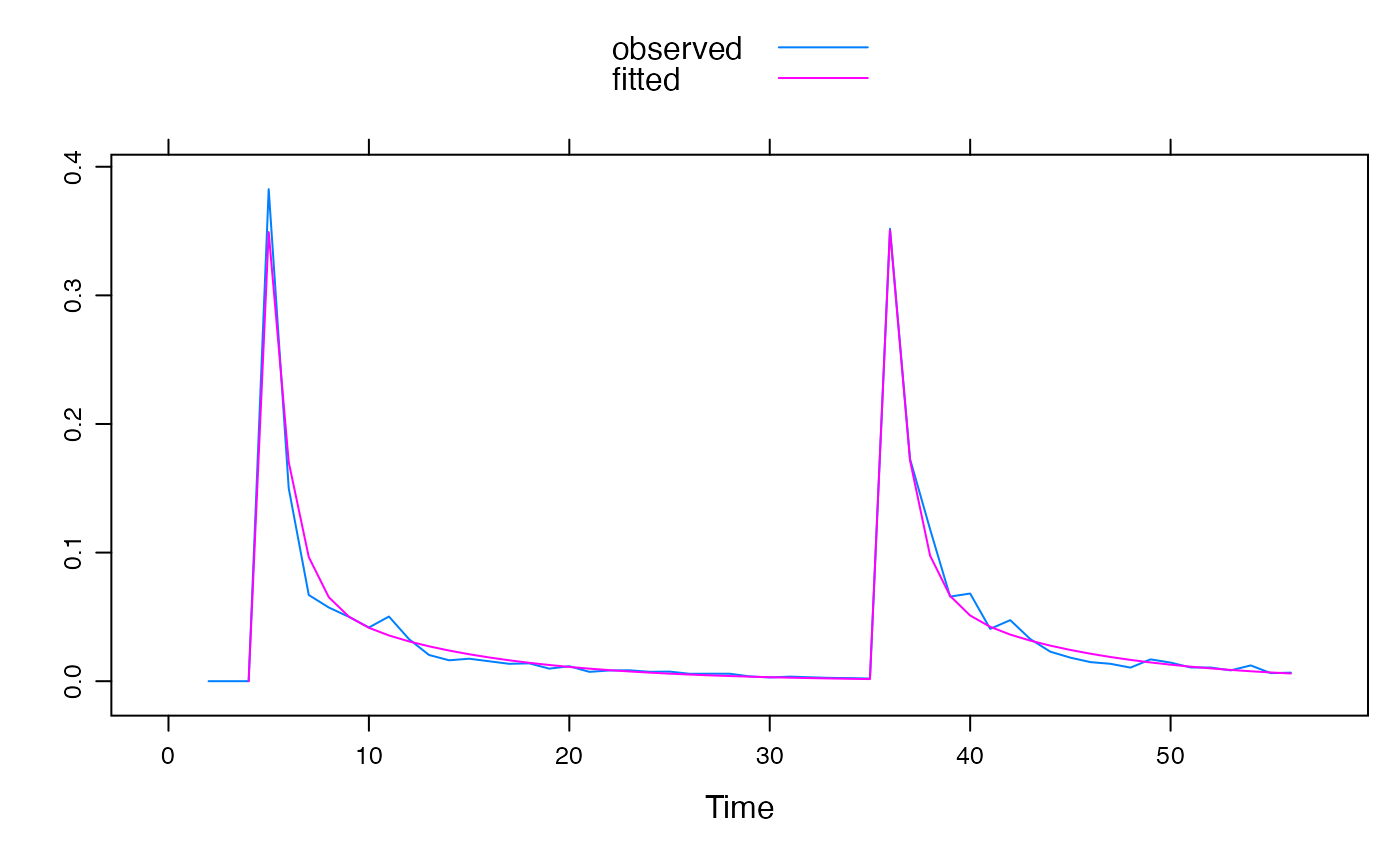
xyplot(ts.union(observed = Yh, fitted = fitted(fit1)),
  superpose = TRUE
)
