Exponential components transfer function models

A unit hydrograph (linear transfer function) defined as a system of exponentially receding components. Each component is defined by its time constant and fractional volume, and if there are multiple (up to 3) such components they may be in a parallel and/or series configuration.

expuh.ls.fit(
  DATA,
  order = hydromad.getOption("order"),
  delay = hydromad.getOption("delay"),
  quiet = FALSE,
  ...
)

Arguments

DATA: Placeholder
order: Placeholder
delay: Placeholder
quiet: Placeholder
...: Placeholder

Value

the model output as a ts object, with the same dimensions and time window as the input U. If return_components = TRUE, it will have multiple columns named Xs, Xq and, if relevant, X3.

Details

The expuh model is a transfer function translating an input time series U into an output series X. It describes a configuration of exponentially decaying components, each defined by a recession rate $\alpha$ and peak response $\beta$. However, in hydrology these parameters are more easily interpreted in terms of time constants $\tau$ (number of time steps to reduce to a fraction $1/e$, 37%) and fractional volumes v. These are directly related as:

$$\tau = -1 / \log(\alpha)$$

$$v = \beta / (1 - \alpha)$$

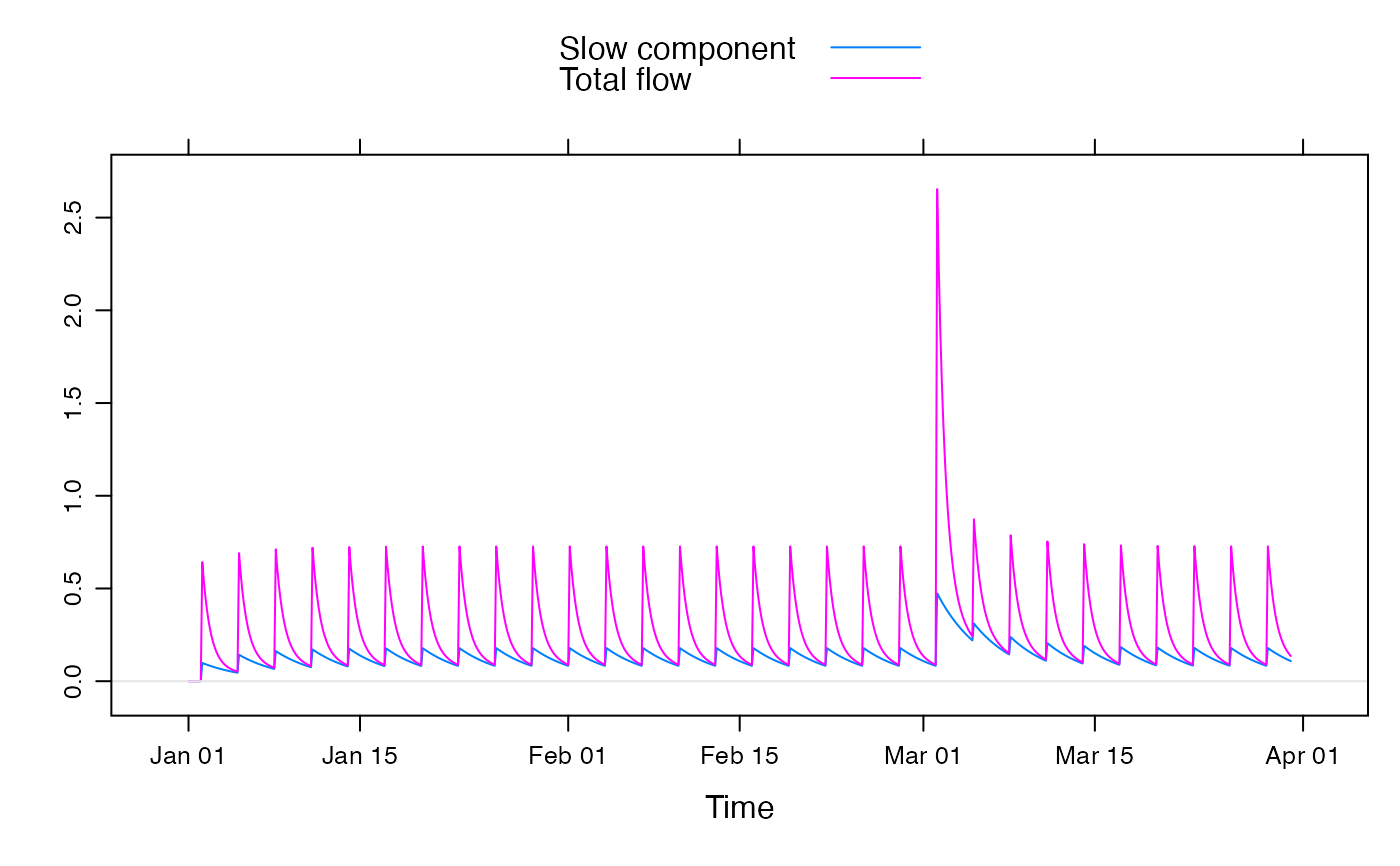
If there are two components in parallel, these are conventionally called slow (s) and quick (q) flow components. The total simulated flow X is the sum of these; $X[t] = X_s[t] + X_q[t]$, and:

$$X_s[t] = \alpha_s X_s[t-1] + \beta_s U[t]$$ $$X_q[t] = \alpha_q X_q[t-1] + \beta_q U[t]$$

Two components might also be arranged in series rather than parallel, in which case:

$$X_s[t] = \alpha_s X_s[t-1] + \beta_s U[t]$$ $$X[t] = \alpha_q X[t-1] + \beta_q X_s[t]$$

This configuration is specified by the argument series = 1. The default series = 0 specifies all components to be in parallel.

In the case of three components, with corresponding time constants $\tau_s$, $\tau_q$ and $tau_3$ (tau_s, tau_q, tau_3), there are four possible types of configuration:

list("series = 0"): all 3 components in parallel, i.e. independent flows: X = s + q + 3. In this case v_q defaults to 1 - v_s - v_3 in order to ensure that the total volume is 1.
list("series = 1"): one component in parallel with two in series: the q component is in series with the 3 component, and the s component is in parallel: X = (q * 3) + s. In this case v_q defaults to 1.
list("series = 2"): two components in parallel with one in series: the s and q components are in parallel and the 3 component is in series: X = 3 * (s + q). In this case v_q defaults to 1 - v_s in order to ensure that the total volume of the parallel component is 1. The total volume will be 1 if v_3 is also 1.
list("series = 3"): all 3 components in series: X = s * q * 3. In this case v_q defaults to 1. The total volume will be 1 if v_s and v_3 are also 1.

References

Jakeman, A.J., I.G. Littlewood, and P.G. Whitehead (1990), Computation of the instantaneous unit hydrograph and identifiable component flows with application to two small upland catchments, Journal of Hydrology, 117: 275-300.

Author

Felix Andrews felix@nfrac.org

Examples


data(HydroTestData)
mod1 <- hydromad(HydroTestData,
  routing = "expuh",
  tau_s = 30, tau_q = 5, v_s = 0.5
)
flowcomps <- predict(mod1, return_components = TRUE)
xyplot(cbind(
  `Slow component` = flowcomps[, "Xs"],
  `Total flow` = flowcomps[, 1] + flowcomps[, 2]
),
superpose = TRUE
) +
  latticeExtra::layer(panel.refline(h = 0))


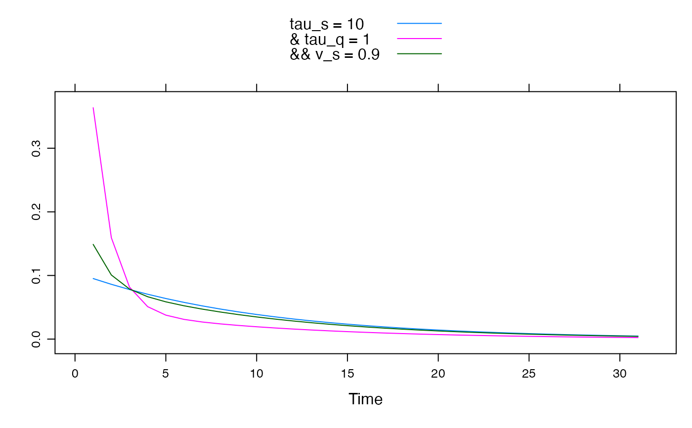
U <- ts(c(1, rep(0, 30)))
xyplot(cbind(
  "tau_s = 10" = expuh.sim(U, tau_s = 10),
  "& tau_q = 1" = expuh.sim(U, tau_s = 10, tau_q = 1, v_s = 0.5),
  "&& v_s = 0.9" = expuh.sim(U, tau_s = 10, tau_q = 1, v_s = 0.9)
),
superpose = TRUE
)