Estimate transfer function models by Simple Refined Instrumental Variables method.

Calibrate unit hydrograph transfer function models (armax or expuh) using Simple Refined Instrumental Variables (SRIV) method.

armax.sriv.fit(
  DATA,
  order = hydromad.getOption("order"),
  delay = hydromad.getOption("delay"),
  noise.order = hydromad.getOption("riv.noise.order"),
  fixed.ar = NULL,
  ...,
  fallback = TRUE,
  na.action = na.pass,
  epsilon = hydromad.getOption("sriv.epsilon"),
  max.iterations = hydromad.getOption("sriv.iterations")
)

Arguments

DATA

a ts-like object with named columns:

list("U")

observed input time series.

list("Q")

observed output time series.

order

the transfer function order. See armax.

delay

delay (lag time / dead time) in number of time steps. If missing, this will be estimated from the cross correlation function.

noise.order

placeholder

fixed.ar

placeholder

...

further arguments may include

prefilter

initX

trace

~~Describe trace here~~

fallback

placeholder

na.action

placeholder

epsilon

placeholder

max.iterations

placeholder (i.e. negative or imaginary poles) are detected.

Value

a tf object, which is a list with components

coefficients

the fitted parameter values.

fitted.values

the fitted values.

residuals

the residuals.

delay

the (possibly fitted) delay time.

Details

In normal usage, one would not call these functions directly, but rather specify the routing fitting method for a hydromad model using that function's rfit argument. E.g. to specify fitting an expuh routing model by SRIV one could write

hydromad(..., routing = "expuh", rfit = "sriv")

which uses the default order, hydromad.getOption("order"), or

hydromad(..., routing = "expuh", rfit = list("sriv", order = c(2,1))).

References

Young, P. C. (2008). The refined instrumental variable method. Journal Européen des Systèmes Automatisés 42 (2-3), 149-179. http://dx.doi.org/10.3166/jesa.42.149-179

Jakeman, A. J., G. A. Thomas and C. R. Dietrich (1991). System Identification and Validation for Output Prediction of a Dynamic Hydrologic Process, Journal of Forecasting 10, pp. 319--346.

Ljung, Lennart (1999). System Identification: Theory for the User (second edition). Prentice Hall. pp. 224-226, 466.

See also

armax, expuh

Author

Felix Andrews felix@nfrac.org

Examples

U <- ts(c(0, 0, 0, 1, rep(0, 30), 1, rep(0, 20)))
Y <- expuh.sim(lag(U, -1), tau_s = 10, tau_q = 2, v_s = 0.5, v_3 = 0.1)
set.seed(0)
Yh <- Y * rnorm(Y, mean = 1, sd = 0.2)
fit1 <- armax.sriv.fit(ts.union(U = U, Q = Yh),
  order = c(2, 2), warmup = 0
)
fit1
#> 
#> Unit Hydrograph / Linear Transfer Function
#> 
#> Call:
#> armax.sriv.fit(DATA = ts.union(U = U, Q = Yh), order = c(2, 2), 
#>     warmup = 0)
#> 
#> Order: (n=2, m=2)  Delay: 1
#> ARMAX Parameters:
#>       a_1        a_2        b_0        b_1        b_2  
#>  1.145551  -0.244799   0.350852  -0.240868  -0.007109  
#> Exponential component parameters:
#>    tau_s     tau_q       v_s       v_q       v_3  
#>  6.69975   0.79487   0.66335   0.40223  -0.02904  
#> TF Structure: S + Q + inst. (three in parallel)
#>     Poles:0.2842, 0.8613
#> 
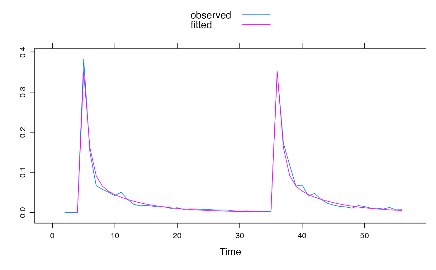
xyplot(ts.union(observed = Yh, fitted = fitted(fit1)),
  superpose = TRUE
)