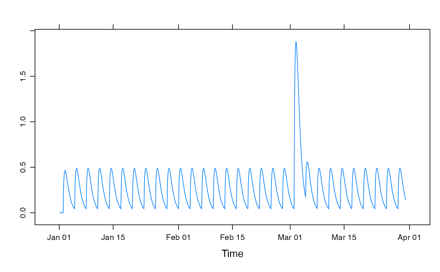
ARMAX linear transfer functions with a single input and single output series. Can be used as a general Unit Hydrograph transfer function, defined by Auto-Regressive and Moving Average coefficients.
armax.sim(
  U,
  a_1 = 0,
  a_2 = 0,
  a_3 = 0,
  b_0 = 1,
  b_1 = 0,
  b_2 = 0,
  b_3 = 0,
  pars = NULL,
  delay = 0,
  init = 0,
  na.action = na.pass,
  epsilon = hydromad.getOption("sim.epsilon"),
  return_components = FALSE
)

ssg.armax(theta)

normalise.armax(theta)
Arguments
- U
input time series.
- a_1, a_2, a_3, b_0, b_1, b_2, b_3
ARMAX coefficients. Auto-regressive terms begin with
aand moving average terms begin withb. See Details section.- pars
the ARMAX coefficients as a named vector. If this is given, it will over-ride the named parmameter arguments. Any number of terms can be given here, it is not limited to the named arguments.
- delay
lag (dead time) between input and response, in time steps.
- init
initial values for the autoregressive filter.
- na.action
function to remove missing values, e.g.
na.omit.- epsilon
values smaller than this will be set to zero.
- return_components
whether to return exponential component time series. If
TRUE, the parameters will be converted to an exponential components formulation, and passed toexpuh.sim. This may fail in some cases.- theta
the parameters as a named vector.
Value
the model output as a ts object, with the same
dimensions and time window as the input U. If
return_components = TRUE, it will have multiple columns named
Xs, Xq and, if relevant, X3.
Details
The transfer function used here, with input u and output x is: $$x[t] = a_1 x[t-1] + \ldots + a_n x[t-n] + $$$$ b_0 u[t-\delta] + \ldots + b_m u[t-m-\delta]$$
and the order is denoted \((n, m)\), with delay \(\delta\).
References
Jakeman, A.J., I.G. Littlewood, and P.G. Whitehead (1990), Computation of the instantaneous unit hydrograph and identifiable component flows with application to two small upland catchments, Journal of Hydrology, 117: 275-300.
