Estimate transfer function models by Inverse Filtering.

Calibrate unit hydrograph transfer function models (armax or expuh) using Inverse Filtering.

armax.inverse.fit(
  DATA,
  order = hydromad.getOption("order"),
  delay = hydromad.getOption("delay"),
  fit.method = hydromad.getOption("inverse.fit.method"),
  normalise = TRUE,
  init.U = TRUE,
  pars = NULL,
  use.Qm = TRUE,
  fft.inverse.sim = FALSE,
  rises.only = FALSE,
  ...,
  max.iterations = hydromad.getOption("inverse.iterations"),
  rel.tolerance = hydromad.getOption("inverse.rel.tolerance"),
  par.epsilon = hydromad.getOption("inverse.par.epsilon"),
  init.attempt = 0,
  trace = hydromad.getOption("trace")
)

Arguments

DATA

a ts-like object with named columns:

list("Q")

observed output time series.

list("P")

observed input time series (optional).

order

the transfer function order. See armax.

delay

delay (lag time / dead time) in number of time steps. If missing, this will be estimated from the cross correlation function.

fit.method

Placeholder

normalise

Placeholder

init.U

Placeholder

pars

Placeholder

use.Qm

Placeholder

fft.inverse.sim

Placeholder

rises.only

Placeholder

...

Placeholder

max.iterations

Placeholder

rel.tolerance

Placeholder

par.epsilon

Placeholder

init.attempt

Placeholder

trace

Placeholder

Value

a tf object, which is a list with components

coefficients

the fitted parameter values.

fitted.values

the fitted values.

residuals

the residuals.

delay

the (possibly fitted) delay time.

Details

In normal usage, one would not call these functions directly, but rather specify the routing fitting method for a hydromad model using that function's rfit argument. E.g. to specify fitting an expuh routing model by inverse filtering one could write

hydromad(..., routing = "expuh", rfit = "inverse")

or

hydromad(..., routing = "expuh", rfit = list("inverse", order = c(2,1))).

References

...

See also

armax.inverse.sim, expuh, armax.sriv.fit

Author

Felix Andrews felix@nfrac.org

Examples

U <- ts(c(0, 0, 0, 1, rep(0, 30), 1, rep(0, 20)))
Y <- expuh.sim(lag(U, -1), tau_s = 10, tau_q = 2, v_s = 0.5, v_3 = 0.1)
set.seed(0)
Yh <- Y * rnorm(Y, mean = 1, sd = 0.2)
fit1 <- armax.inverse.fit(ts.union(P = U, Q = Yh),
  order = c(2, 2), warmup = 0
)
#> Warning: did not converge after 12 iterations
fit1
#> 
#> Unit Hydrograph / Linear Transfer Function
#> 
#> Call:
#> armax.inverse.fit(DATA = ts.union(P = U, Q = Yh), order = c(2, 
#>     2), warmup = 0)
#> 
#> Order: (n=2, m=2)  Delay: 1
#> ARMAX Parameters:
#>       a_1        a_2        b_0        b_1        b_2  
#>  1.148917  -0.246043   0.348228  -0.247966  -0.003136  
#> Exponential component parameters:
#>    tau_s     tau_q       v_s       v_q       v_3  
#>  6.85247   0.79598   0.62715   0.38560  -0.01275  
#> TF Structure: S + Q + inst. (three in parallel)
#>     Poles:0.2847, 0.8642
#> 
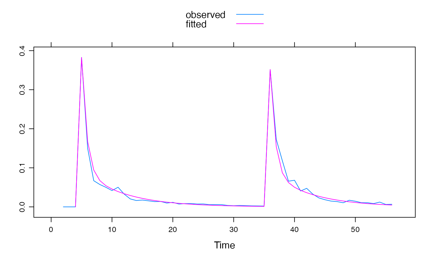
xyplot(ts.union(observed = Yh, fitted = fitted(fit1)),
  superpose = TRUE
)