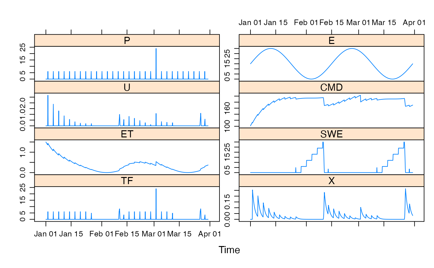
Simple degree day factor snow model

Simple degree day factor snow model coupled with IHACRES CMD soil moisture model.

snow.sim(
  DATA,
  Tmax,
  Tmin,
  kd,
  kf,
  rcap,
  Tmelt = Tmin,
  cr = 1,
  cs = 1,
  LSWE_0 = 0,
  ISWE_0 = 0,
  ...,
  return_state = FALSE
)

Arguments

DATA

a ts-like object with named columns:

list("P")

time series of areal rainfall depths, usually in mm.

list("E")

time series of potential evapo-transpiration, or more typically, temperature as an indicator of this.

Tmax

temperature threshold for rain, all rain is liquid above this threshold.

Tmin

temperature threshold for rain, all rain is snow below this threshold.

kd

degree day factor for snowmelt.

kf

degree day factor for freezing.

rcap

retention parameter for liquid water capacity of snowpack.

Tmelt

temperature threshold for snowmelt and freezing in the snowpack.

cr

correction factor for rainfall.

cs

correction factor for snowfall.

LSWE_0, ISWE_0

initial values of state variables.

...

parameters for the IHACRES.CMD.model.

return_state

to return state variables as well as the effective rainfall.

Value

snow.sim returns the modelled time series of effective rainfall, or if return_state = TRUE, a multi-variate time series with named columns U (effective rainfall), SWE (snow water equivalent) and TF, as well as the CMD state variables.

Details

SWE snow water equivalent

ISWE water equivalent of ice in the snowpack

LSWE liquid water retained in the snowpack

References

Kokkonen T., Jakeman A.J, Koivusalo.H, Norton.J.: COMPUTATIONAL METHODS FOR WATER RESOURCE ASSESSMENTS: AN EXERCISE KIT Educational Series on Modelling and Software iEMSs International Modelling and Software Society Available through www.iemss.org

See also

hydromad(sma = "snow") to work with models as objects (recommended).

Author

Coded in R by Jarkko Koskela @tkk.fi 2010-02-26.

Converted to C by Felix Andrews felix@nfrac.org.

Examples

## view default parameter ranges:
str(hydromad.options("snow"))
#> List of 1
#>  $ snow:List of 10
#>   ..$ Tmax: num [1:2] 0 2
#>   ..$ Tmin: num [1:2] -1 1
#>   ..$ cr  : num [1:2] 0.8 2
#>   ..$ cs  : num [1:2] 0.8 2
#>   ..$ kd  : num [1:2] 2 5
#>   ..$ kf  : num [1:2] 0 2
#>   ..$ rcap: num [1:2] 0 1
#>   ..$ f   : num [1:2] 0.01 3
#>   ..$ e   : num [1:2] 0.01 1.5
#>   ..$ d   : num 200

data(HydroTestData)
mod0 <- hydromad(HydroTestData, sma = "snow", routing = "expuh")
mod0
#> 
#> Hydromad model with "snow" SMA and "expuh" routing:
#> Start = 2000-01-01, End = 2000-03-31
#> 
#> SMA Parameters:
#>       lower upper     
#> Tmax   0.00   2.0     
#> Tmin  -1.00   1.0     
#> cr     0.80   2.0     
#> cs     0.80   2.0     
#> kd     2.00   5.0     
#> kf     0.00   2.0     
#> rcap   0.00   1.0     
#> f      0.01   3.0     
#> e      0.01   1.5     
#> d    200.00 200.0 (==)
#> Routing Parameters:
#> NULL

## simulate with some arbitrary parameter values
mod1 <- update(mod0,
  Tmax = 15, Tmin = 5, cr = 1, cs = 1,
  kd = 3, kf = 1, rcap = 0.5,
  d = 200, f = 0.5, e = 0.1, tau_s = 10
)

## plot results with state variables
testQ <- predict(mod1, return_state = TRUE)
xyplot(cbind(HydroTestData[, 1:2], snow = testQ))


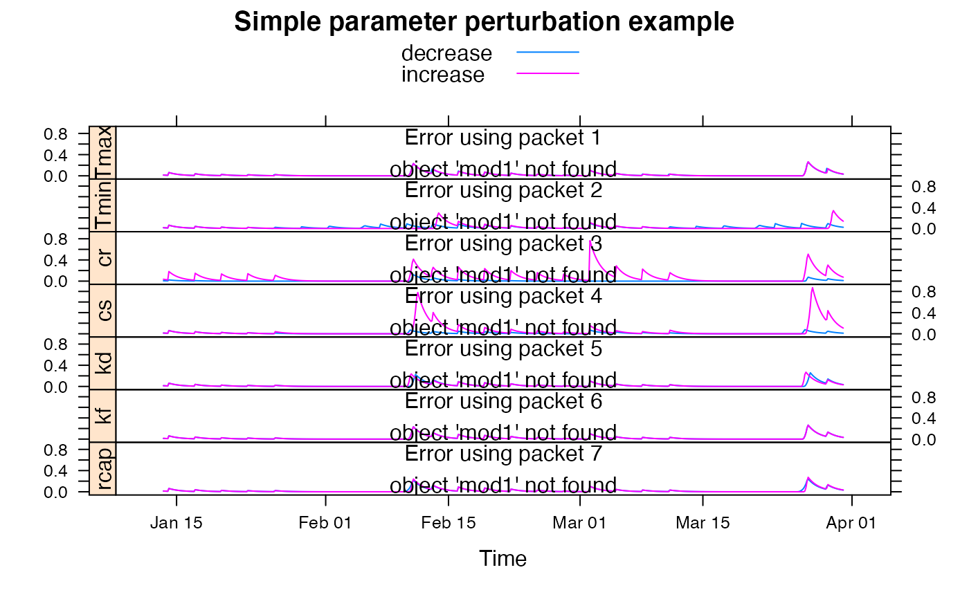
## show effect of increase/decrease in each parameter
parlist <- list(
  Tmax = c(10, 20), Tmin = c(0, 10),
  cr = c(0.5, 2), cs = c(0.5, 2),
  kd = c(2, 5), kf = c(0, 2), rcap = c(0, 1)
)
parsims <- mapply(
  val = parlist, nm = names(parlist),
  FUN = function(val, nm) {
    lopar <- min(val)
    hipar <- max(val)
    names(lopar) <- names(hipar) <- nm
    fitted(runlist(
      decrease = update(mod1, newpars = lopar),
      increase = update(mod1, newpars = hipar)
    ))
  }, SIMPLIFY = FALSE
)

xyplot.list(parsims,
  superpose = TRUE, layout = c(1, NA),
  strip = FALSE, strip.left = TRUE,
  main = "Simple parameter perturbation example"
) +
  latticeExtra::layer(panel.lines(fitted(mod1), col = "grey", lwd = 2))