IHACRES Catchment Moisture Deficit (CMD) model

The Catchment Moisture Deficit (CMD) effective rainfall model for IHACRES. It is a conceptual-type model, where input rainfall is partitioned explicitly into drainage, evapo-transpiration, and changes in catchment moisture.

cmd.sim(DATA, f, e, d, shape = 0, M_0 = d/2, return_state = FALSE)

Arguments

DATA

a ts-like object with named columns:

list("P"): time series of areal rainfall depths, usually in mm.
list("E"): time series of potential evapo-transpiration, or more typically, temperature as an indicator of this.

f

CMD stress threshold as a proportion of d.

e

temperature to PET conversion factor.

d

CMD threshold for producing flow.

shape

defines form of the $dU/dP$ relationship: shape = 0 is the linear form, shape = 1 is the trigonometric form, and shape > 1 is the power form.

M_0

starting CMD value.

return_state

to return state variables as well as the effective rainfall.

Value

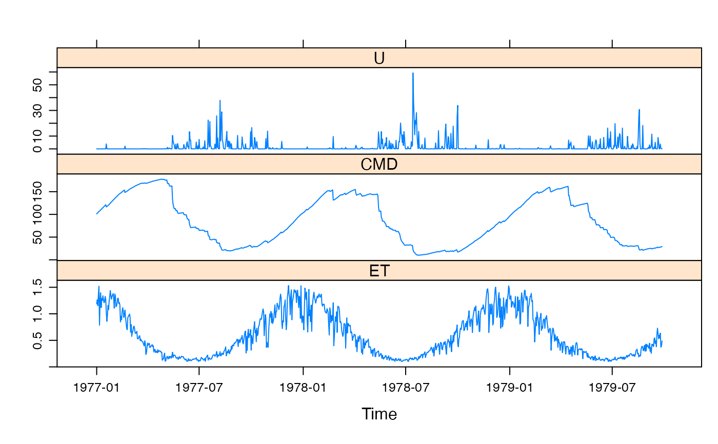
cmd.sim returns the modelled time series of effective rainfall, or if return_state = TRUE, a multi-variate time series with named columns U (effective rainfall), CMD and ET(evapo-transpiration $E_T$).

Details

The mass balance step is: $$M[t] = M[t-1] - P[t] + E_T[t] + U[t]$$

where $M$ represents catchment moisture deficit (CMD), constrained below by 0 (the nominal fully saturated level). P is catchment areal rainfall, $E_T$ is evapo-transpiration, and U is drainage (effective rainfall). All are, typically, in units of mm per time step.

Rainfall effectiveness (i.e. drainage proportion) is a simple instantaneous function of the CMD, with a threshold at $M = d$. In the default linear form this is:

$$\frac{\mathrm{d}U}{\mathrm{d}P} = 1 - \min(1, M/d)$$

The trigonometric form is

$$\frac{\mathrm{d}U}{\mathrm{d}P} = 1 - \min(1, \sin^2(\pi M / 2d))$$

The power form is

$$\frac{\mathrm{d}U}{\mathrm{d}P} = 1 - \min(1, (M/d)^a)$$ where a = 10 ^ (shape / 50)

The actual drainage each time step involves the integral of these relations.

Evapo-transpiration is also a simple function of the CMD, with a threshold at $M = f d$: $$E_T[t] = e E[t] \min(1, \exp\left(2\left(1 - \frac{M_f}{fd}\right)\right))$$

Note that the evapo-transpiration calculation is based on $M_f$, which is the CMD after precipitation and drainage have been accounted for.

Note

Normally compiled C code is used for simulation, but if return_state = TRUE a slower implementation in R is used.

References

Croke, B.F.W. and A.J. Jakeman (2004), A Catchment Moisture Deficit module for the IHACRES rainfall-runoff model, Environmental Modelling and Software, 19(1): 1-5.

Croke, B.F.W. and A.J. Jakeman (2005), Corrigendum to ``A Catchment Moisture Deficit module for the IHACRES rainfall-runoff model'' [Environ. Model. Softw. 19 (1) (2004) 1-5], Environmental Modelling and Software, 20(7): 977.

Author

Felix Andrews felix@nfrac.org

Examples


## view default parameter ranges:
str(hydromad.options("cmd"))
#> List of 1
#>  $ cmd:List of 4
#>   ..$ f    : num [1:2] 0.01 3
#>   ..$ e    : num [1:2] 0.01 1.5
#>   ..$ d    : num [1:2] 50 550
#>   ..$ shape: num 0

data(Canning)
x <- cmd.sim(Canning[1:1000, ],
  d = 200, f = 0.7, e = 0.166,
  return_state = TRUE
)
xyplot(x)


data(HydroTestData)
mod0 <- hydromad(HydroTestData, sma = "cmd", routing = "expuh")
mod0
#> 
#> Hydromad model with "cmd" SMA and "expuh" routing:
#> Start = 2000-01-01, End = 2000-03-31
#> 
#> SMA Parameters:
#>       lower upper     
#> f      0.01   3.0     
#> e      0.01   1.5     
#> d     50.00 550.0     
#> shape  0.00   0.0 (==)
#> Routing Parameters:
#> NULL

## simulate with some arbitrary parameter values
mod1 <- update(mod0, d = 200, f = 0.5, e = 0.1, tau_s = 10)

## plot results with state variables
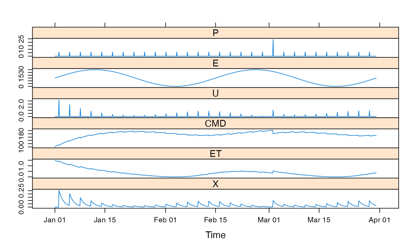
testQ <- predict(mod1, return_state = TRUE)
xyplot(cbind(HydroTestData[, 1:2], cmd = testQ))


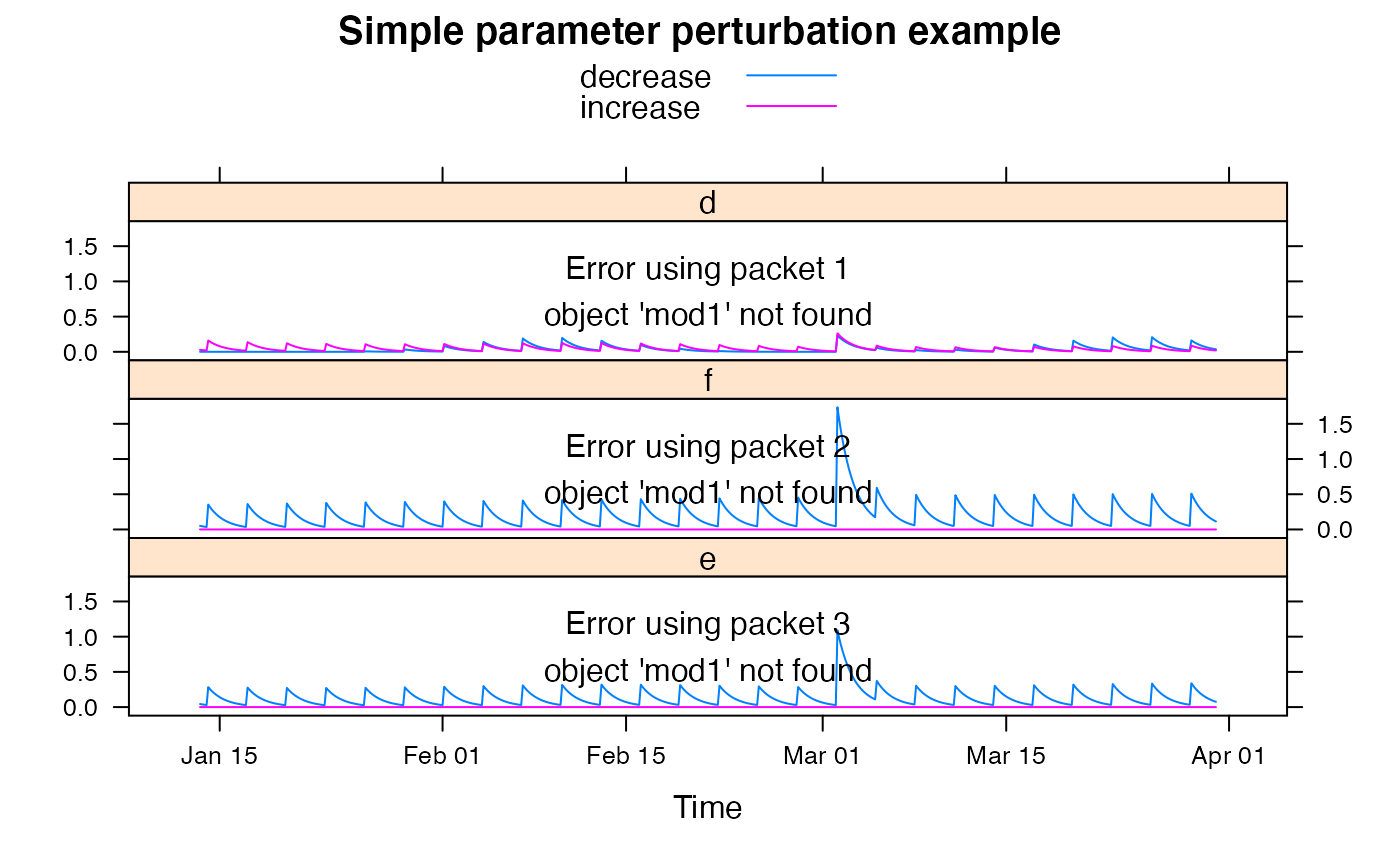
## show effect of increase/decrease in each parameter
parlist <- list(
  d = c(50, 550), f = c(0.01, 3),
  e = c(0.01, 1.5)
)
parsims <- mapply(
  val = parlist, nm = names(parlist),
  FUN = function(val, nm) {
    lopar <- min(val)
    hipar <- max(val)
    names(lopar) <- names(hipar) <- nm
    fitted(runlist(
      decrease = update(mod1, newpars = lopar),
      increase = update(mod1, newpars = hipar)
    ))
  }, SIMPLIFY = FALSE
)

xyplot.list(parsims,
  superpose = TRUE, layout = c(1, NA),
  main = "Simple parameter perturbation example"
) +
  latticeExtra::layer(panel.lines(fitted(mod1), col = "grey", lwd = 2))