Australian Water Balance Model (AWBM)

Australian Water Balance Model (AWBM): simple 3 bucket model.

awbm.sim(
  DATA,
  cap.ave,
  cap1 = 0.01 * cap.ave/area1,
  cap2 = 0.33 * cap.ave/area2,
  cap3 = 0.66 * cap.ave/area3,
  area2 = 0.433,
  area3 = 0.433,
  area1 = 1 - area2 - area3,
  etmult = 1,
  S1_0 = 0,
  S2_0 = 0,
  S3_0 = 0,
  return_state = FALSE
)

Arguments

DATA

time-series-like object with columns P (precipitation, mm) and E (potential evapo-transpiration, mm).

cap.ave

average soil water storage capacity (mm). This is not used directly in the model, but rather to define default values of the other parameters.

cap1, cap2, cap3

soil water storage capacities (mm) for the three fractional areas.

area1, area2, area3

fractional areas with corresponding capacities. These must sum to 1.

etmult

multiplier for the E input data.

S1_0, S2_0, S3_0

initial soil moisture levels (mm).

return_state

to return the soil moisture levels S1, S2 and S3 together with effective rainfall U.

Value

the simulated effective rainfall, a time series of the same length as the input series.

Details

This is a very simple model: saturation excess from three buckets with different capacities are added together with fractional areas for weights.

This is the soil moisture accounting component; the model described in the literature has a two-store routing component also, with parameters BFI, \(K_b\) and \(K_s\). These correspond directly to the expuh routing model parameters v_s, tau_s and tau_q, so the full model can be specified as:

hydromad(..., sma = "awbm", routing = "expuh", rfit = list("sriv", order = c(2, 1)))

References

Boughton, W. (2004). The australian water balance model. Environmental Modelling & Software 19 (10), 943-956. http://dx.doi.org/10.1016/j.envsoft.2003.10.007

See also

hydromad(sma = "awbm") to work with models as objects (recommended).

Author

Felix Andrews felix@nfrac.org

Examples

## view default parameter ranges:
str(hydromad.options("awbm"))
#> List of 1
#>  $ awbm:List of 2
#>   ..$ cap.ave: num [1:2] 1 1000
#>   ..$ etmult : num [1:2] 0.01 1

data(HydroTestData)
mod0 <- hydromad(HydroTestData, sma = "awbm", routing = "expuh")
mod0
#> 
#> Hydromad model with "awbm" SMA and "expuh" routing:
#> Start = 2000-01-01, End = 2000-03-31
#> 
#> SMA Parameters:
#>         lower upper  
#> cap.ave  1.00  1000  
#> etmult   0.01     1  
#> Routing Parameters:
#> NULL

## simulate with some arbitrary parameter values
mod1 <- update(mod0, cap.ave = 40, etmult = 0.1, tau_s = 10)

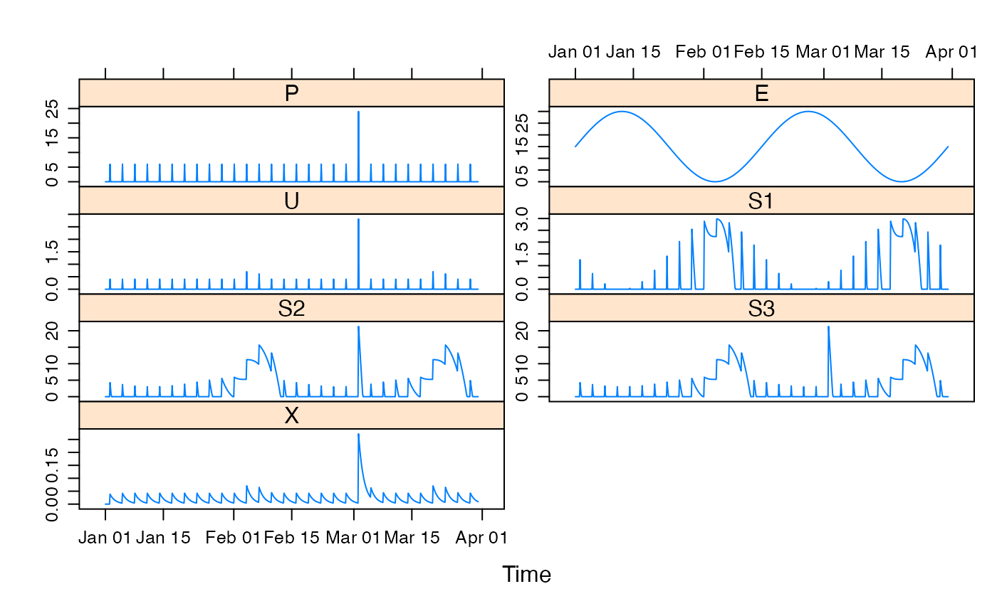
## plot results with state variables
testQ <- predict(mod1, return_state = TRUE)
xyplot(cbind(HydroTestData[, 1:2], awbm = testQ))


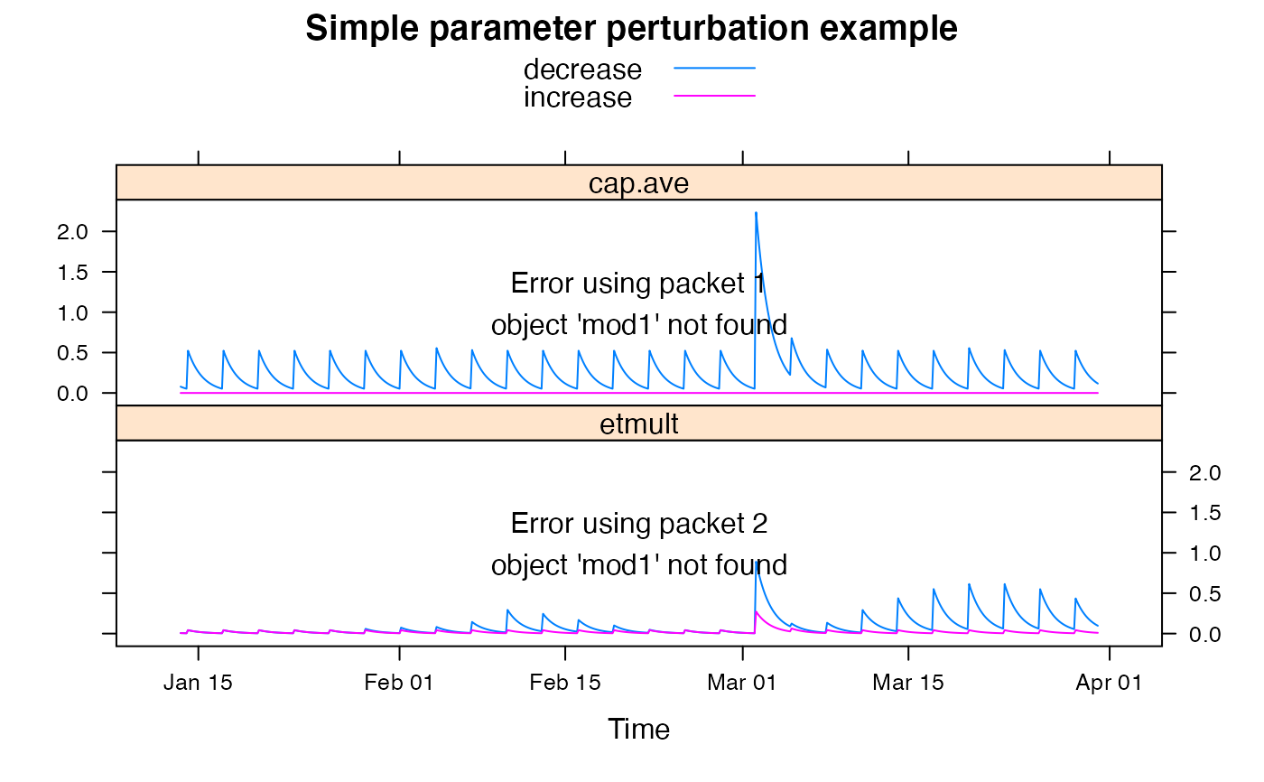
## show effect of increase/decrease in each parameter
parRanges <- list(cap.ave = c(1, 1000), etmult = c(0.01, 1))
parsims <- mapply(
  val = parRanges, nm = names(parRanges),
  FUN = function(val, nm) {
    lopar <- min(val)
    hipar <- max(val)
    names(lopar) <- names(hipar) <- nm
    fitted(runlist(
      decrease = update(mod1, newpars = lopar),
      increase = update(mod1, newpars = hipar)
    ))
  }, SIMPLIFY = FALSE
)

xyplot.list(parsims,
  superpose = TRUE, layout = c(1, NA),
  main = "Simple parameter perturbation example"
) +
  latticeExtra::layer(panel.lines(fitted(mod1), col = "grey", lwd = 2))