Time series sensitivity analysis

Generic method to evaluate sensitivity analysis methods in decoupled mode (see tell) on a time series of results, as produced for example by evalParsRollapply. See examples for more details.

tellTS(
  x,
  ts.matrix,
  fun,
  indices,
  parallel = hydromad.getOption("parallel")[["tellTS"]],
  ...
)

Arguments

x

A sensitivity analysis object for which results still need to be provided. A typed list storing the state of the sensitivity study (parameters, data, estimates), as returned by sensitivity analyses objects constructors, such as morris, sobol2002, etc.

ts.matrix

A matrix of model responses, with each row corresponding to the parameter sets identified in x and each column a timestep for which to evaluate sensitivity indices. If the matrix does not fit in memory, ff matrices are also supported.

fun

A function fun(i,x) which returns a data.frame, where i is the index of the time series and x is a complete sensitivity analysis object, i.e. the result of calling tell(x,y). For sobol2002 and sobol2007, the default is to return the Total Sensitivity Index (TSI) and its minimum and maximum bootstrap confidence interval.

indices

(Optional) Which time indices to use. By default, sensitivity indices are calculated for all columns of ts.matrix

parallel

If "clusterApply", evaluate parameters in parallel using the parallel or snow package. See hydromad_parallelisation

...

Ignored by default implementation

Value

a data.frame with columns produced by fun

References

Herman, J. D., P. M. Reed, and T. Wagener. 2013. "Time-Varying Sensitivity Analysis Clarifies the Effects of Watershed Model Formulation on Model Behavior." Water Resources Research 49 (3): 1400-1414. doi: 10.1002/wrcr.20124

See also

hydromad_sensitivity for sensitivity analysis on static rather than time series model output, evalParsRollapply to obtain parameter sets

Author

Joseph Guillaume

Examples

library(sensitivity)

## Load data
data(Cotter)
obs <- Cotter[1:1000]

## Define rainfall-runoff model structure
model.str <- hydromad(obs,
  sma = "cwi", routing = "expuh",
  tau_q = c(0, 2), tau_s = c(2, 100), v_s = c(0, 1)
)

## Set the random seed to obtain replicable results
set.seed(19)

## Setup Morris Sensitivity analysis
incomplete <- morris(
  ## Names of factors/parameters
  factors = names(getFreeParsRanges(model.str)),
  ## Number of repetitions
  r = 4,
  ## List specifying design type and its parameters
  design = list(type = "oat", levels = 10, grid.jump = 2),
  ## Minimum value of each non-fixed parameter
  binf = sapply(getFreeParsRanges(model.str), min),
  ## Maximum value of each non-fixed parameter
  bsup = sapply(getFreeParsRanges(model.str), max)
)


# Calculate rolling time series of objective for each parameter set,
#   keeping results in memory
runs <- evalParsRollapply(incomplete$X, model.str,
  objective = ~ hmadstat("r.squared")(Q, X) /
    (2 - hmadstat("r.squared")(Q, X)),
  parallel = "none",
  filehash.name = NULL
)
#> Running 24 model evaluations with parallelisation='none'

# Calculate Morris elementary effects for each timestep
sens <- tellTS(incomplete, runs, parallel = "none")
#> Calculating sensitivity on 871 data points with parallelisation

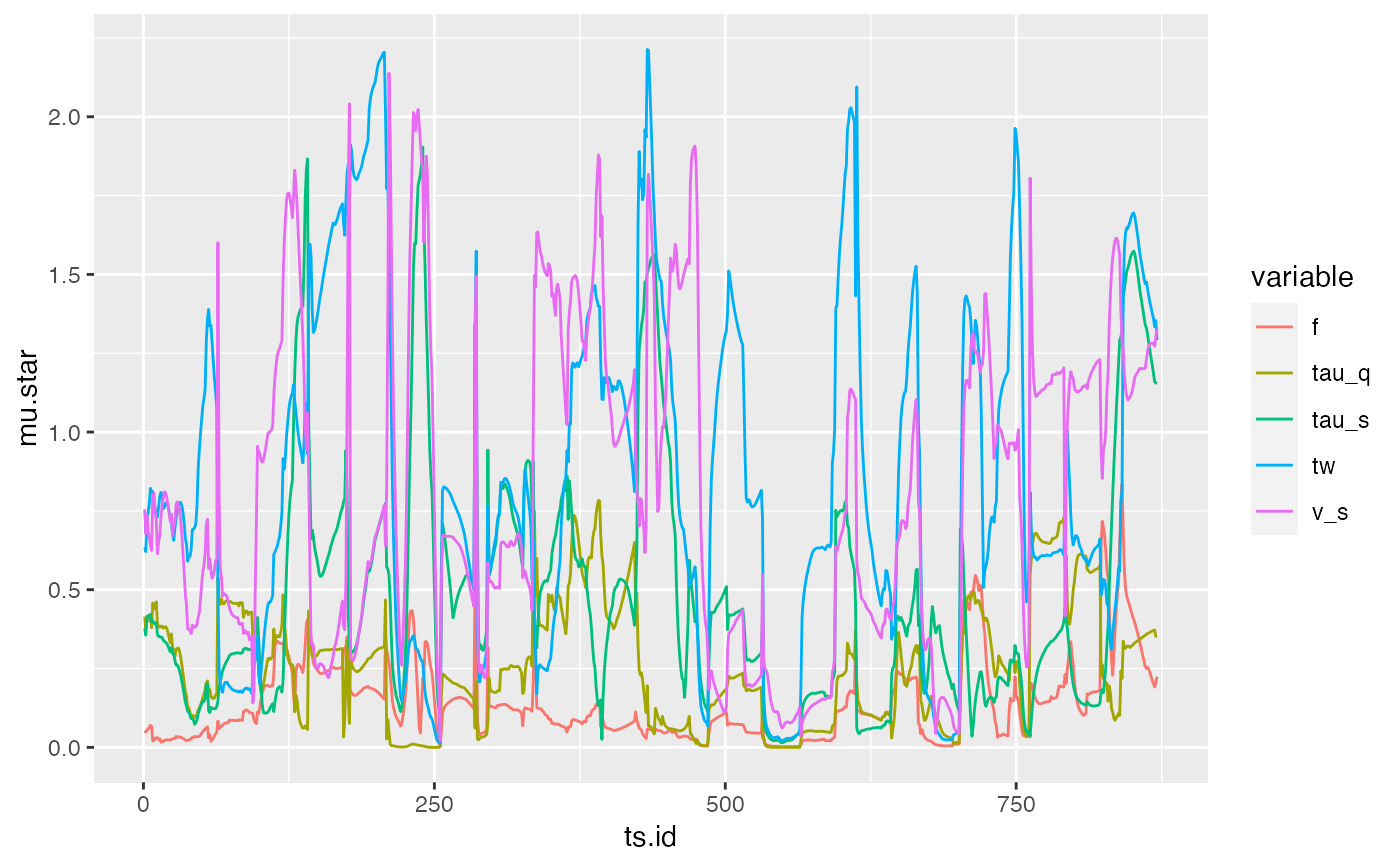
## Plot time series of mean absolute elementary effects
library(ggplot2)
#> 
#> Attaching package: ‘ggplot2’
#> The following object is masked from ‘package:latticeExtra’:
#> 
#>     layer
qplot(x = ts.id, y = mu.star, colour = variable, data = sens, geom = "line")


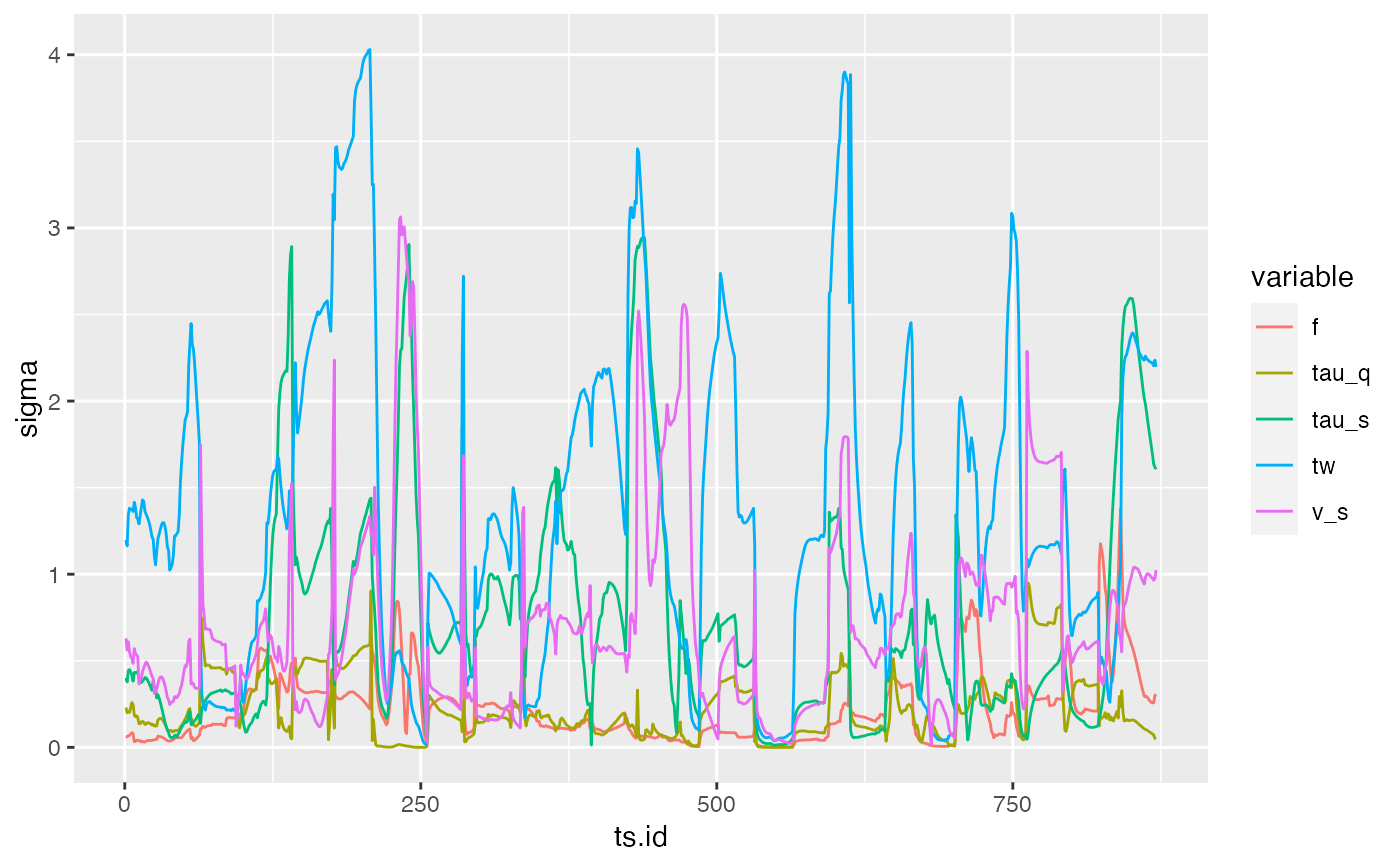
## And of standard deviation of elementary effects
qplot(x = ts.id, y = sigma, colour = variable, data = sens, geom = "line")


######################################################################
if (FALSE) {
## Sobol indices
### Setup parallelisation
library(parallel)
hydromad.options("parallel" = list("evalParsRollapply" = "clusterApply"))
hydromad.options("parallel" = list("tellTS" = "clusterApply"))
cl <- makeCluster(3)
clusterEvalQ(cl, library(hydromad))

### Create sobol design
n <- 1000 ## Set number of samples desired
X1 <- parameterSets(getFreeParsRanges(model.str), n)
X2 <- parameterSets(getFreeParsRanges(model.str), n)
incomplete <- sobol2002(model = NULL, X1 = X1, X2 = X2, nboot = 100)

### Run model for each parameter set, storing result to disk
system.time(runs <- evalParsRollapply(incomplete$X, model.str,
  objective = hmadstat("r.squared"), parallel = "clusterApply"
))

## Calculate sobol indices for each timestep with stored runs
system.time(TSI <- tellTS(incomplete, runs))

## Plot time series of sensitivities
library(ggplot2)
qplot(x = ts.id, y = original, colour = variable, data = TSI, geom = "line")

## Time series plot facetted by variable showing bootstrapped confidence interval
ggplot(data = TSI) +
  geom_ribbon(aes(
    x = ts.id, ymin = get("min. c.i."),
    ymax = get("max. c.i.")
  ), fill = "grey") +
  geom_line(aes(x = ts.id, y = original)) +
  facet_wrap(~variable)
}