Simple time-varying runoff proportion

Simple time-varying runoff proportion. Rainfall is scaled by the runoff coefficient estimated in a moving window. This SMA uses streamflow data, so can not be used for prediction.

runoffratio.sim(
  DATA,
  width = 30,
  kernel = 2,
  sides = 2,
  rrthresh = 0,
  qlag = 0,
  scale = 1,
  return_state = FALSE
)

Arguments

DATA

time-series-like object with columns P (precipitation) and Q (streamflow).

width

width of the time window (in time steps) in which to estimate the runoff coefficient.

kernel

type of window used to estimate the runoff coefficient: 1 is rectangular, 2 is triangular-weighted, 3 is Gaussian-like.

sides

2 for time-centered estimates, 1 for estimates using data backward in time only.

rrthresh

a theshold value of the runoff ratio, below which there is no effective rainfall.

qlag

number of time steps to lag the streamflow (relative to rainfall) before estimating the runoff coefficient.

scale

constant multiplier of the result, for mass balance. If this parameter is set to NA (as it is by default) in hydromad it will be set by mass balance calculation.

return_state

ignored.

Value

the simulated effective rainfall, a time series of the same length as the input series.

See also

hydromad(sma = "runoffratio") to work with models as objects (recommended).

Author

Felix Andrews felix@nfrac.org

Examples

## view default parameter ranges:
str(hydromad.options("runoffratio"))
#> List of 1
#>  $ runoffratio:List of 2
#>   ..$ rrthresh: num [1:2] 0 0.2
#>   ..$ scale   : logi NA

data(HydroTestData)
mod0 <- hydromad(HydroTestData, sma = "runoffratio", routing = "expuh")
mod0
#> 
#> Hydromad model with "runoffratio" SMA and "expuh" routing:
#> Start = 2000-01-01, End = 2000-03-31
#> 
#> SMA Parameters:
#>          lower upper  
#> rrthresh     0   0.2  
#> scale       NA    NA  
#> Routing Parameters:
#> NULL

## simulate with some arbitrary parameter values
mod1 <- update(mod0, width = 30, rrthresh = 0.2, tau_s = 10)

## plot results with state variables
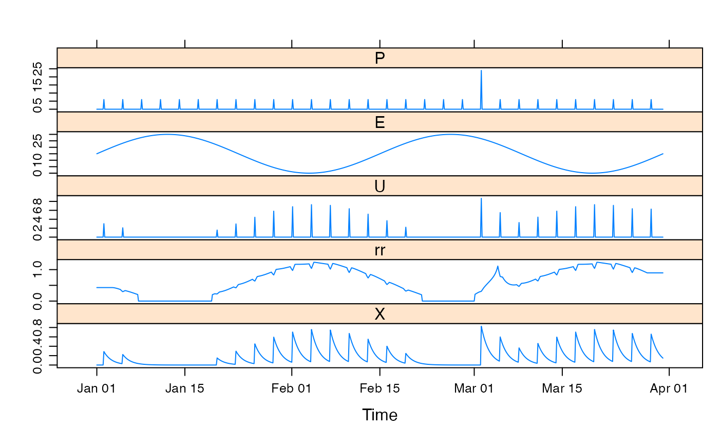
testQ <- predict(mod1, return_state = TRUE)
xyplot(cbind(HydroTestData[, 1:2], runoffratio = testQ))


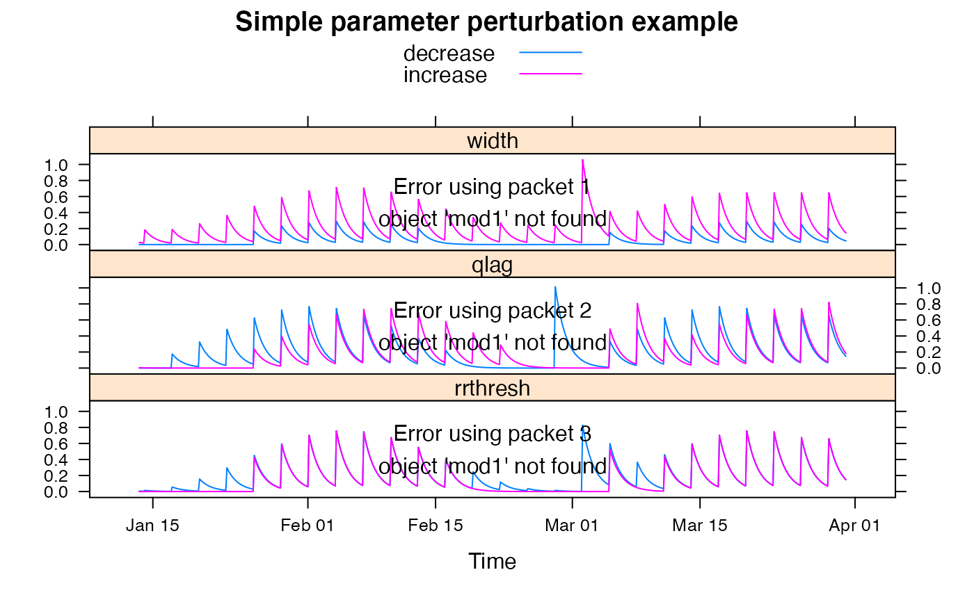
## show effect of increase/decrease in each parameter
parRanges <- list(
  width = c(10, 180), qlag = c(-30, 30),
  rrthresh = c(0, 0.5)
)
parsims <- mapply(
  val = parRanges, nm = names(parRanges),
  FUN = function(val, nm) {
    lopar <- min(val)
    hipar <- max(val)
    names(lopar) <- names(hipar) <- nm
    fitted(runlist(
      decrease = update(mod1, newpars = lopar),
      increase = update(mod1, newpars = hipar)
    ))
  }, SIMPLIFY = FALSE
)

xyplot.list(parsims,
  superpose = TRUE, layout = c(1, NA),
  main = "Simple parameter perturbation example"
) +
  latticeExtra::layer(panel.lines(fitted(mod1), col = "grey", lwd = 2))