Fit a hydromad model using the SCE (Shuffled Complex Evolution) algorithm.

Fit a hydromad model using the SCE (Shuffled Complex Evolution) algorithm.

fitBySCE(
  MODEL,
  objective = hydromad.getOption("objective"),
  control = hydromad.getOption("sce.control"),
  vcov = FALSE
)

Arguments

MODEL

a model specification created by hydromad. It should not be fully specified, i.e one or more parameters should be defined by ranges of values rather than exact values.

objective

objective function to maximise, given as a function(Q, X, ...). See objFunVal.

control

settings for the SCE algorithm. See SCEoptim. Note that unlike SCEoptim, the objective function is maximised (fnscale=-1) by default.

vcov

if vcov = TRUE, the parameter variance-covariance matrix will be estimated from the final population. It can be extract using vcov.

Value

the best model from those sampled, according to the given objective function. Also, these extra elements are inserted:

fit.result

the result from SCEoptim.

objective

the objective function used.

funevals

total number of evaluations of the model simulation function.

timing

timing vector as returned by system.time.

See also

SCEoptim, objFunVal

Author

Felix Andrews felix@nfrac.org

Examples

data(Cotter)
x <- Cotter[1:1000]

## IHACRES CWI model with power law unit hydrograph
modx <- hydromad(x, sma = "cwi", routing = "powuh")
modx
#> 
#> Hydromad model with "cwi" SMA and "powuh" routing:
#> Start = 1966-05-01, End = 1969-01-24
#> 
#> SMA Parameters:
#>       lower upper     
#> tw        0   100     
#> f         0     8     
#> scale    NA    NA     
#> l         0     0 (==)
#> p         1     1 (==)
#> t_ref    20    20 (==)
#> Routing Parameters:
#>   lower upper  
#> a  0.01    60  
#> b  0.50     3  
#> c  0.50     2  

## run with cut-down settings (for a speedy example only!)
foo <- fitBySCE(modx, control = list(maxit = 5, ncomplex = 2))
#> Warning: Maximum number of function evaluations or iterations reached.

summary(foo)
#> 
#> Call:
#> hydromad(DATA = x, sma = "cwi", routing = "powuh", a = 4.96111, 
#>     b = 1.0574, c = 1.43395, tw = 97.6414, f = 6.6972, scale = 0.00135911)
#> 
#> Time steps: 900 (0 missing).
#> Runoff ratio (Q/P): (0.7028 / 2.285) = 0.3075
#> rel bias: -1.504e-16
#> r squared: 0.7374
#> r sq sqrt: 0.8245
#> r sq log: 0.8139
#> 
#> For definitions see ?hydromad.stats
#> 

## return value from SCE:
str(foo$fit.result)
#> List of 11
#>  $ call       : language SCEoptim(FUN = do_sce, par = initpars, lower = lower, upper = upper, control = control)
#>  $ control    :List of 13
#>   ..$ ncomplex  : num 2
#>   ..$ cce.iter  : logi NA
#>   ..$ fnscale   : num -1
#>   ..$ elitism   : num 1
#>   ..$ initsample: chr "latin"
#>   ..$ reltol    : num 1e-05
#>   ..$ tolsteps  : num 7
#>   ..$ maxit     : num 5
#>   ..$ maxeval   : num Inf
#>   ..$ maxtime   : num Inf
#>   ..$ returnpop : logi FALSE
#>   ..$ trace     : num 0
#>   ..$ REPORT    : num 1
#>  $ par        : Named num [1:5] 4.96 1.06 1.43 97.64 6.7
#>   ..- attr(*, "names")= chr [1:5] "a" "b" "c" "tw" ...
#>  $ value      : num -0.847
#>  $ convergence: num 1
#>  $ message    : chr "Maximum number of function evaluations or iterations reached."
#>  $ counts     : num 254
#>  $ iterations : num 5
#>  $ time       : num 6.49
#>  $ POP.FIT.ALL: num [1:5, 1:22] -0.829 -0.83 -0.839 -0.841 -0.847 ...
#>  $ BESTMEM.ALL: num [1:5, 1:5] 8.6 9.3 3.53 1.73 4.96 ...
#>   ..- attr(*, "dimnames")=List of 2
#>   .. ..$ : NULL
#>   .. ..$ : chr [1:5] "a" "b" "c" "tw" ...
#>  - attr(*, "class")= chr [1:2] "SCEoptim" "list"

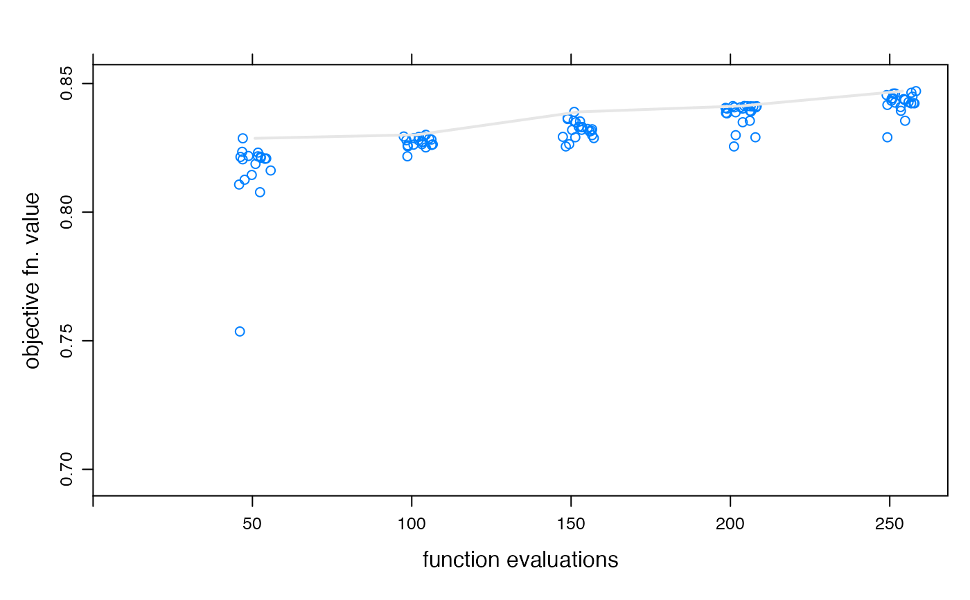
## plot objective function value convergence over time
xyplot(optimtrace(foo, raw = TRUE),
  screens = 1, type = "p",
  jitter.x = TRUE, ylim = c(0.7, NA), xlim = c(0, NA),
  xlab = "function evaluations", ylab = "objective fn. value"
) +
  latticeExtra::layer(panel.average(..., horiz = FALSE, fun = max, lwd = 2))