Fit a hydromad model using the DE (Differential Evolution) algorithm.

Fit a hydromad model using the DE (Differential Evolution) algorithm.

fitByDE(
  MODEL,
  objective = hydromad.getOption("objective"),
  control = hydromad.getOption("de.control")
)

Arguments

MODEL

a model specification created by hydromad. It should not be fully specified, i.e one or more parameters should be defined by ranges of values rather than exact values.

objective

objective function to maximise, given as a function(Q, X, ...). See objFunVal.

control

settings for the DE algorithm. See DEoptim.control.

Value

the best model from those sampled, according to the given objective function. Also, these extra elements are inserted:

fit.result

the result from DEoptim.

objective

the objective function used.

funevals

total number of evaluations of the model simulation function.

timing

timing vector as returned by system.time.

See also

DEoptim, objFunVal

Author

Felix Andrews felix@nfrac.org

Examples

library("DEoptim")
#> Loading required package: parallel
#> 
#> DEoptim package
#> Differential Evolution algorithm in R
#> Authors: D. Ardia, K. Mullen, B. Peterson and J. Ulrich

data(Cotter)
x <- Cotter[1:1000]

## IHACRES CWI model with power law unit hydrograph
modx <- hydromad(x, sma = "cwi", routing = "powuh")
modx
#> 
#> Hydromad model with "cwi" SMA and "powuh" routing:
#> Start = 1966-05-01, End = 1969-01-24
#> 
#> SMA Parameters:
#>       lower upper     
#> tw        0   100     
#> f         0     8     
#> scale    NA    NA     
#> l         0     0 (==)
#> p         1     1 (==)
#> t_ref    20    20 (==)
#> Routing Parameters:
#>   lower upper  
#> a  0.01    60  
#> b  0.50     3  
#> c  0.50     2  

foo <- fitByDE(modx, control = DEoptim.control(itermax = 5))

summary(foo)
#> 
#> Call:
#> hydromad(DATA = x, sma = "cwi", routing = "powuh", a = 8.4263, 
#>     b = 1.25033, c = 1.76043, tw = 96.2573, f = 5.15738, scale = 0.00131429)
#> 
#> Time steps: 900 (0 missing).
#> Runoff ratio (Q/P): (0.7028 / 2.285) = 0.3075
#> rel bias: -3.69e-18
#> r squared: 0.7309
#> r sq sqrt: 0.8295
#> r sq log: 0.8256
#> 
#> For definitions see ?hydromad.stats
#> 

## return value from DE:
str(foo$fit.result)
#> List of 2
#>  $ optim :List of 4
#>   ..$ bestmem: Named num [1:5] 8.43 1.25 1.76 96.26 5.16
#>   .. ..- attr(*, "names")= chr [1:5] "a" "b" "c" "tw" ...
#>   ..$ bestval: num -0.851
#>   ..$ nfeval : int 12
#>   ..$ iter   : int 5
#>  $ member:List of 6
#>   ..$ lower    : Named num [1:5] 0.01 0.5 0.5 0 0
#>   .. ..- attr(*, "names")= chr [1:5] "a" "b" "c" "tw" ...
#>   ..$ upper    : Named num [1:5] 60 3 2 100 8
#>   .. ..- attr(*, "names")= chr [1:5] "a" "b" "c" "tw" ...
#>   ..$ bestmemit: num [1:5, 1:5] 10.99 10.99 10.99 10.99 8.43 ...
#>   .. ..- attr(*, "dimnames")=List of 2
#>   .. .. ..$ : chr [1:5] "1" "2" "3" "4" ...
#>   .. .. ..$ : chr [1:5] "a" "b" "c" "tw" ...
#>   ..$ bestvalit: num [1:5] -0.842 -0.842 -0.847 -0.847 -0.851
#>   ..$ pop      : num [1:50, 1:5] 12.4 25.7 10.5 24.9 13.2 ...
#>   ..$ storepop : list()
#>  - attr(*, "class")= chr "DEoptim"

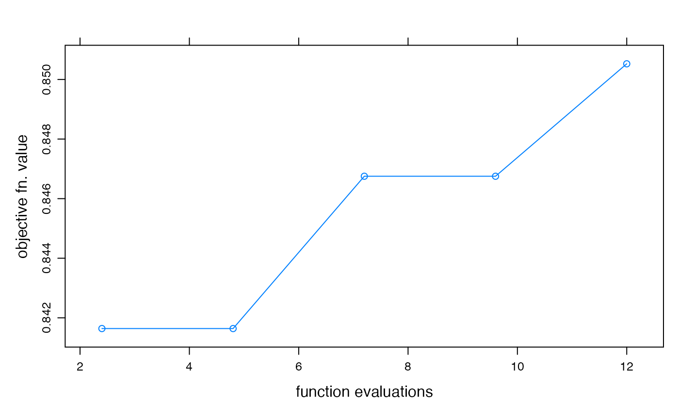
## plot objective function value convergence over time
xyplot(optimtrace(foo),
  type = "b",
  xlab = "function evaluations", ylab = "objective fn. value"
)