Single-bucket Soil Moisture Accounting models

Single-bucket Soil Moisture Accounting models with saturated/unsaturated zones and interception.

bucket.sim(
  DATA,
  Sb,
  fc = 1,
  a.ei = 0,
  M = 0,
  a.ss = 0,
  etmult = 1,
  S_0 = 0.5,
  return_state = FALSE
)

Arguments

DATA

time-series-like object with columns P (precipitation, mm) and E (potential evapo-transpiration, mm).

Sb

Maximum soil water storage (mm).

fc

Field capacity (0 - 1).

a.ei

Interception coefficient (\(\alpha_{ei}\)).

M

Fraction of catchment area covered by deep rooted vegetation.

a.ss

Recession coefficients for subsurface flow from saturated zone (\(\alpha_{ss}\)).

etmult

Multiplier for the E input data.

S_0

Initial soil moisture level as a fraction of Sb.

return_state

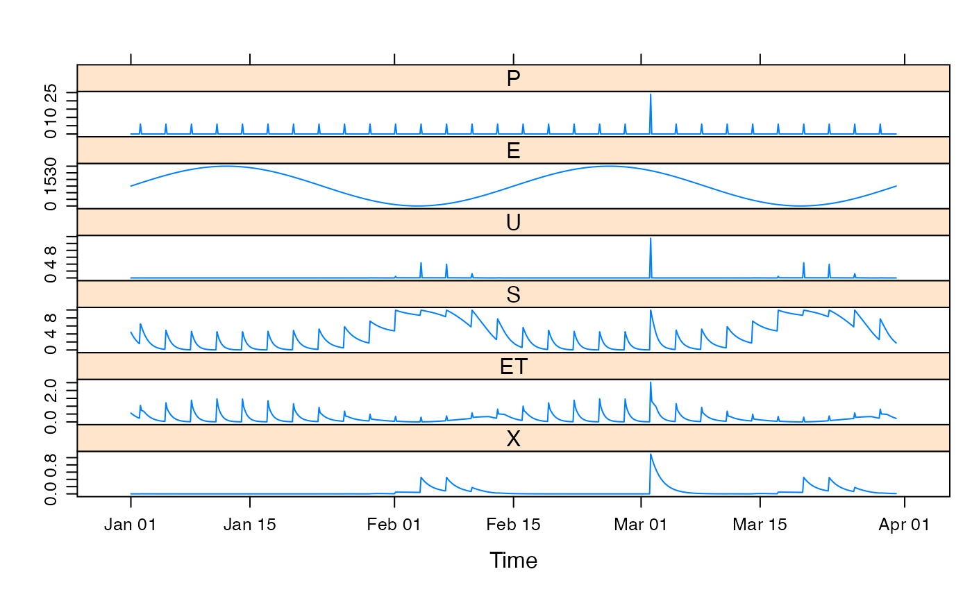
to return the series U, S and ET (evapotranspiration).

Value

the simulated effective rainfall, a time series of the same length as the input series.

Details

From formulations given in Bai et. al. (2009), which were based on Farmer et. al. (2003).

The general mass balance structure is: $$dS/dt = p - q(S) - e(S, Ep)$$

The default parameter ranges were also taken from Bai et. al. (2009).

References

Farmer, D., M. Sivapalan, Farmer, D. (2003). Climate, soil and vegetation controls upon the variability of water balance in temperate and semiarid landscapes: downward approach to water balance analysis. Water Resources Research 39(2), p 1035.

Bai, Y., T. Wagener, P. Reed (2009). A top-down framework for watershed model evaluation and selection under uncertainty. Environmental Modelling and Software 24(8), pp. 901-916.

See also

hydromad(sma = "bucket") to work with models as objects (recommended).

Author

Felix Andrews felix@nfrac.org

Examples

## view default parameter ranges:
str(hydromad.options("bucket"))
#> List of 1
#>  $ bucket:List of 5
#>   ..$ Sb  : num [1:2] 0.1 1200
#>   ..$ fc  : num [1:2] 0.01 1
#>   ..$ a.ei: num [1:2] 0 0.49
#>   ..$ M   : num [1:2] 0 1
#>   ..$ a.ss: num [1:2] 0 0.5

data(HydroTestData)
mod0 <- hydromad(HydroTestData, sma = "bucket", routing = "expuh")
mod0
#> 
#> Hydromad model with "bucket" SMA and "expuh" routing:
#> Start = 2000-01-01, End = 2000-03-31
#> 
#> SMA Parameters:
#>      lower   upper  
#> Sb    0.10 1200.00  
#> fc    0.01    1.00  
#> a.ei  0.00    0.49  
#> M     0.00    1.00  
#> a.ss  0.00    0.50  
#> Routing Parameters:
#> NULL

## simulate with some arbitrary parameter values
mod1 <- update(mod0,
  Sb = 10, fc = 0.5, M = 0.5, etmult = 0.05,
  a.ei = 0.05, a.ss = 0.01, tau_s = 10
)
## plot results with state variables
testQ <- predict(mod1, return_state = TRUE)
xyplot(cbind(HydroTestData[, 1:2], bucket = testQ))


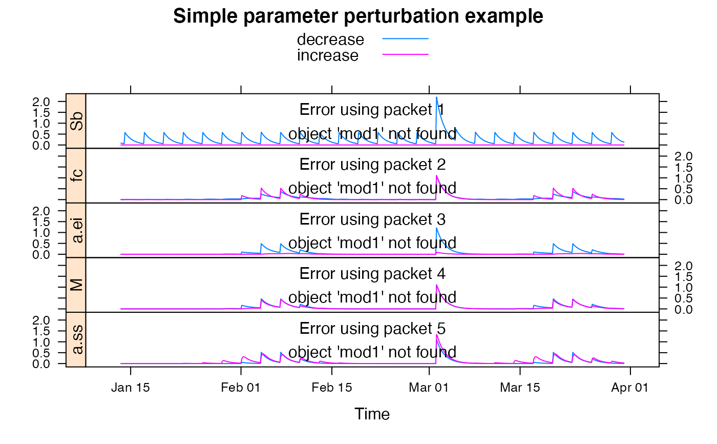
## show effect of increase/decrease in each parameter
parRanges <- hydromad.getOption("bucket")
parsims <- mapply(
  val = parRanges, nm = names(parRanges),
  FUN = function(val, nm) {
    lopar <- min(val)
    hipar <- max(val)
    names(lopar) <- names(hipar) <- nm
    fitted(runlist(
      decrease = update(mod1, newpars = lopar),
      increase = update(mod1, newpars = hipar)
    ))
  }, SIMPLIFY = FALSE
)

xyplot.list(parsims,
  superpose = TRUE, layout = c(1, NA),
  strip = FALSE, strip.left = TRUE,
  main = "Simple parameter perturbation example"
) +
  latticeExtra::layer(panel.lines(fitted(mod1), col = "grey", lwd = 2))